Nonlinear Dynamics as Non-Parametric Regression

Disclaimer: This material is more or less copied in whole cloth from Chapter 26 of Cosma Shalizi's fantastic Advanced Data Analysis from an Elementary Point of View. Only the model system has been changed.

As I mentioned before, many of the ideas from the nonlinear dynamics community appear very similar to ideas developed in the statistical community for the analysis of nonlinear time series¹. Cosma commented briefly on using nonlinear regression for such problems in the lecture two days ago, and I thought I'd code up some examples to make sure I really understood the ideas.

First, the statistical model. The simplest regression method for time series is a linear autoregressive model: you assume the future dynamics of a system are some linear function of the past dynamics, plus noise. That is, if we denote the trajectory of our system (stochastic process) as \(\{ X_{t}\}_{t = 1}^{\infty}\), then we assume that \[ X_{t} = \alpha + \sum_{j = 1}^{p} \beta_{j} X_{t - j} + \epsilon_{t}\] where \(E\left[\epsilon_{t} | X_{t-p}^{t-1}\right] = 0\) and \(\text{Var}\left[\epsilon_{t} | X_{t-1}^{t-p}\right] = \sigma^{2},\) and we generally assume that the residuals \(\epsilon_{t}\) are uncorrelated with each other and the inputs². For those who have taken a statistical methods course, this should look a lot of like linear regression. Hence the name linear auto (self) regression.

This methodology only works well when the linear assumptions holds. If we look at lag plots (i.e. plot \(X_{t}\) vs. \(X_{t-1}\)), we should get out a noisy line. If we don't, then the dynamics aren't linear, and we should probably be a bit more clever.

One stab at being clever is to assume an additive model for the dynamics (before, we assumed a linear additive model). That is, we can assume that the dynamics are given by \[ X_{t} = \alpha + \sum_{j = 1}^{p} f_{j}(X_{t - j}) + \epsilon_{t}\] where the \(f_{j}\) can be arbitrary functions that we'll try to learn from the data. This will capture nonlinearities, but not associations between the different lags. If we wanted to, we could include cross terms, but let's start by adding this simple nonlinearity.

It's worth noting that we've implicitly assumed that the process we're trying to model is conditionally stationary. In particular, we've assumed that the conditional mean \[E[X_{t} | X_{t - p}^{t-1}] = \alpha + \sum_{j = 1}^{p} f_{j}(X_{t - j})\] only depends on the value of \(X_{t-p}^{t-1}\), not on the time index \(t\). This assumption gets encoded by the fact that we try to learn the functions \(f_{j}\) using all of the data, and assume they don't change over time. This is a fairly weak form of stationarity (and one that doesn't get much mention), but it's also all we need to do prediction. If the process is really non-stationary, then without some reasonable model for how the process changes over time, we won't be able to do much. So be it.

Fortunately, there's already an R package, gam, for doing all of the fun optimization that makes additive models work. R is truly an amazing thing.

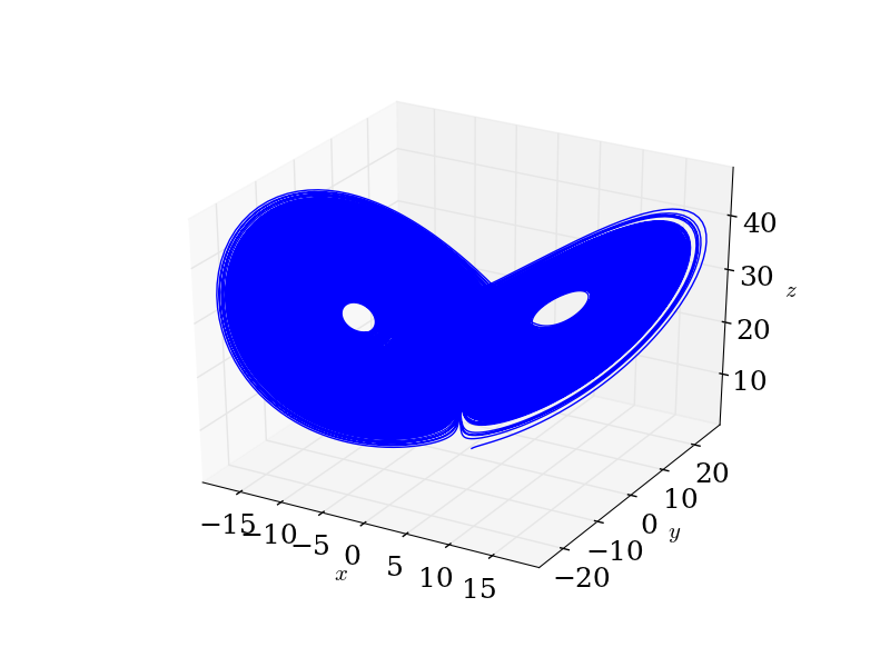
Let's use the Lorenz system as our example, \[ \begin{array}{l} x' &= \sigma (y - x)\\ y' &= x(\rho - z) - y\\ z' &= xy - \beta z \end{array}\] I generated a trajectory (without noise) from this system in the usual way, but now I'll pretend I've just been handed the time series, with no knowledge of the dynamics that created it³.

As a first step, we should plot our data:

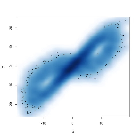
Looks like the Lorenz system. To convince ourselves that a linear autoregressive method won't work particularly well, let's look at a lag one plot:

Again, if the system were truly linear, this should look like a noisy line. It clearly doesn't (we see the attractor sneaking out). Ignore the two colored dots. The blue are the true points, the red our my estimates. But we'll get to that soon.

I'll use a order 5 autoregressive model. That is, I'll assume we're dealing with \[ X_{t} = \alpha + \sum_{j = 1}^{5} f_{j}(X_{t - j}) + \epsilon_{t}\] and try to infer the appropriate \(f_{j}\). As good statisticians / machine learners, if we really care about the predictive ability of our method, we should split our data into a training set and a testing set⁴. Here's how we perform on the training set:

Blue is the true trajectory. Red is our predicted trajectory. And here's how we perform on the testing set:

Not bad. Of course, we're only ever doing single-step ahead prediction. Since there really is a deterministic function mapping us from our current value to the future value (even if we can never write it down), we expect to be able to predict a single step ahead. This is, after all, what I used approximated by using an ODE solver. Let's look at the partial response functions for each of the lags:

The partial response plots play the same roles as the coefficients in a linear model⁵. They tell us how the new value \(X_{t}\) depends on the previous values \(X_{t-5}^{t-1}\). Clearly this relationship isn't linear. We wouldn't expect it to be for the Lorenz system.

Let's see how linear autoregressive model does. Again, let's use fifth order model, so we'll take \[ X_{t} = \alpha + \sum_{j = 1}^{5} \beta_{j} X_{t - j} + \epsilon_{t}.\]

Here's how we perform on the training set:

And on the testing set:

For full disclosure (and because numbers are nice), the mean squared error on the test set was 3.1 and 73.1 using the additive autoregressive and linear autoregressive models, respectively. Clearly the (nonlinear) additive model wins.

I should really choose the order \(p\) using something like cross-validation. For example, we see from the partial response functions that for order 5, the fifth lag is nearly flat: it doesn't seem to contribute much to our prediction. It might stand to reason that we shouldn't try to infer out that far, then. Adding unnecessary complexity to our model makes it more likely that we'll infer structure that isn't there.

With this very simple example⁶, we already see the power of using nonlinear methods. As Shalizi often points out, there's really no principled reason to use linear methods anymore. The world is nonlinear, and we have the technology to deal with that.

Speaking of the technology, I've posted the R code here, and the data file here. The code isn't well-commented, and is mostly adapted from Shalizi's Chapter 26. But it does give a good starting place.

As with most uses of the phrase 'nonlinear,' this one deserves some extra explanation. Here, we use nonlinear to refer to the generating equations, not the observed behavior. Just as linear differential equations give rise to nonlinear trajectories (i.e. sines and cosines, as a special case), linear difference equations give rise to nonlinear maps. Not many (any?) people care about when the observed dynamics are linear: it's easy to predict a trajectory lying on a straight line. Thus, when we say 'linear dynamics' or 'nonlinear dynamics,' we refer to the equations generating that dynamics, not the dynamics themselves. Confusing? Yes. But also unavoidable.↩
We can relax these last few assumptions and get more sophisticated models.↩
If I did have a good reason to believe I had a good model for the system, I'd be better off using a parametric model like a nonlinear variant of the Kalman filter. I've had some experience with this.↩
If I were really a good statistician, I would use cross-validation. But it's a Saturday night, and I'm already avoiding a party I should be at. So you'll have to forgive me.↩
"It's true that a set of plots for \(f_{j}\)s takes more room than a table of \(\beta_{j}\)s, but it's also nicer to look at. There are really very, very few situations when, with modern computing power, linear models are superior to additive models."↩
No offense intended towards Ed Lorenz. I mostly mean simple to implement.↩

Cosma's Greatest Hits

I had the good fortune to attend four lectures by Cosma Shalizi over the past two days. As anyone who has been so unlucky as to listen to me rant about statistics knows, Cosma is one of my academic idols¹. I know him mostly through his research, his blog, and his pedagogical efforts. I've had the pleasure of corresponding with him via email a few times.

As a groupie of sorts, I noticed a few recurring topics in his talks that I'll record here for posterity. With tongue firmly in cheek, I'll call these Cosma's Greatest Hits. These are paraphrases, but I think they get the point across.

Introductory statistics and experimental methods courses are terrible. No wonder many scientists proudly flaunt their hatred of statistics. Modern statistics is cool. And even physicists should learn more about it.
MaxEnt isn't magic. And if you really want the unbiased, maximum entropy estimator, just use the data.
Big data without theory is lame. We can't defeat the curse of dimensionality with more data. Inferring things from high dimensional data is intrinsically hard, and we'll have to be clever to get anything useful out of the data.
\(R^2\) is a dumb metric of goodness of fit. If we care about prediction, why not report mean-squared error on a testing set²?
Linear regression for its own sake is silly. Unless we have a good theory supporting a linear model, we have better tools. The world is not linear: it's about time we started accepting that fact.
Bootstrapping is pretty damn cool.
Asymptotic goodness-of-fit estimators are nice. But at the end of the day, cross-validation works much better.
Machine learning is computational statistics that only cares about predictive ability.
Correlation isn't causation. But we have ways to get at causation now.
(He didn't get to talk about this, but...) Power laws aren't everywhere. And 'scientists' should stop fitting lines to log-log plots and learn some undergraduate statistics.

Some have even called him my 'math crush.'↩
In response to a question about how we should go about changing the culture around linear regression and \(R^{2}\), Cosma responded, "Well, it's not as if we can give The Elements of Statistical Learning to your clients and expect them to read it."↩

Predictive Reading

I often start a book not knowing if I'll finish it. I have a graveyard (more kindly called a bookshelf) full of books that aren't quite completed. This is a nasty habit. Can I do anything to improve it?

I'm currently reading The Fractalist by Benoit Mandelbrot. So far, I've spent an hour and five minutes reading the book. If history is any indication, I'll finish it in another four hours and thirty minutes.

What do I mean? Determining the amount of reading time¹ to complete a book should be a straightforward prediction problem. The data are all there. How many pages have you read? How long did it take to read those pages? How many pages remain? With these three pieces of information, estimating the amount of time to complete a book is a matter of simple extrapolation: how many minutes, at my reading rate, will it take to read the remaining pages? A very simple word problem, indeed.

Of course, this only becomes simple if we can find a simple functional relationship between the time spent reading and the number of pages read. I'm not a machine (?), but the different pages of a pleasure²-reading book are more or less the same in terms of grammatical structure, vocabulary, and content-difficulty. (I'm not reading James Joyce's Ulysses.) Thus, there should be some consistency in the number of pages I read in a given interval of time.

Fortunately, I've been recording the amount of time it takes me to read a given number of pages for a given book since December 2012³. Here is a sample of this data for nine books I've read over the past six months:

As you can see, the number of pages I read in a minute is more or less linear⁴ as a function of the amount of time I spend reading. This linear form is consistent across books. The only thing that changes is the slope of the line.

This, of course, also makes sense. Different books will have different font sizes, different content difficulty, etc., which should result in differing reading rates. Which makes the concept of a fixed 'reading rate' a bit nebulous⁵.

The problem with my current approach is that with each new book, I start the prediction problem from scratch. Basically, I have the model \[ Y_{i} = \beta t_{i} + \epsilon_{i},\] where \(Y_{i}\) is the number of pages I've read on the \(i^{\text{th}}\) reading, \(t_{i}\) is the amount of time spent during that reading, \(\epsilon_{i}\) is a fudge factor, and \(\beta\) is my reading rate for a given book. The problem is that, a priori, I don't know how different my reading rate will be on the new book compared to previous books I've read. One way to get around this is to use a mixed-effect model, and assume that my reading rate on a book is some combination of an intrinsic reading rate plus a book-specific reading rate, \[ \beta = \beta_{\text{book}} + \beta_{\text{intrinsic}}.\] (This seems like a reasonable model to me.) I can then use the previous books to inform my guess at \(\beta_{\text{intrinsic}}\), and then estimate \(\beta_{\text{book}}\) from scratch. This is very similar to empirical Bayes, where we use prior information (collected empirically!) to get a better guess at some parameter.

I'd have to spend more time thinking about how to do this type of analysis formally. But that time would be better spent reading these books. So for now, my crude completion estimator will have to do.

As opposed to the number of calendar days. That's a question of behavioral control. Which, presumably, should be made easier with good data. A common pattern from control theory is that we must first be able to accurately monitor a system before we can control it. This applies to life just as much as it does to factories.↩
As opposed to a technical books. A good rule of thumb: never read a math textbook as if you're reading a novel.↩
Has it only been that long? I can't believe I've lived so much of my life in the dark, unable to predict how much more time I would need to commit to a book to complete it.↩
Except, perhaps, for very short amounts of time spent reading. There are myriad explanations for this: I haven't gotten 'in the zone,' the measurements are noisy at shorter reading times (differences across pages haven't had a chance to average out, time measurements are off, etc.).↩
Much like the idea of a fixed intelligence quotient.↩

The 'Statistician' Loved by Silver

We could let N go to the limit immediately (before taking observations). Now no real thing is infinite. There never has been, nor will there ever be, an infinite number of anything, hence there cannot be an infinite number of observations of anything. In other words, there is just is no real need for notions of infinity. Not for any problem met by man. Which means we'll go to infinity anyway, but only to please the mathematicians who must turn probability into math.

— William Briggs, from Subjective Versus Objective Bayes (Versus Frequentism): Part Final: Parameters!

Briggs is the statistician¹ that Nate Silver cites in The Signal and the Noise for his 'paper' stating that we should no longer teach frequentist statistics.

I'll get to that paper in a bit. But first, let's parse what Briggs's claim. '[T]here is just is no real need for notions of infinity.' Kronecker would be proud. But our notions about these things have advanced a bit since the 1800s. And even if they hadn't, sometimes it can be useful to use continuous approximations, or to take limits. So even if you think the universe is discrete on all levels (Planck lengths and Planck times, and all that physics), we can still find uses for the infinite.

So, Briggs has a disdain for mathematics. Which I would have once thought was an odd opinion for a statistician to have. But I've since learned that some want to turn statistics into an empirical science. Which seems a bit daft to me. Like a dog chasing its tail.

Back to his paper.

Since none but the devout want math, skip it or minimize it. We will not lack for students: even without a saturation of mathematics, those who hear the call will still enter the fold. Since civilians want to understand uncertainty, teach it. This is our great forgotten purpose.

I've been known to claim that we should only teach statistics to those who have earned a black belt in mathematics. Statistics is hard, subtle, and counterintuitive. But it's rarely taught that way. Students taking a STAT100-style course are, of course, already intimidated by basic arithmetic. But I don't think we should water down the material. Instead, we should improve basic math education so that students might rise to the occasion.

At the same time, Briggs notes that we need to teach these people something if they have any hope of getting along in quantitative fields (or even just in society). I don't have a good answer for this. I feel like more harm than good is often done with introductory statistics classes. But I don't think students would leave a course centered around Bayesian statistics with all that much more subtle of a view on the subject.

Recovery of these courses is important because there are lot of folks out there who, because they once had a graduate survey course in regression, and have personally produced a p-value or two, feel they are versed sufficiently in probability to pass on their skills to fresh students. But their rendering of the subtleties of the subject is often not unlike the playing of a worn cassette tape, which itself was copied from a bootleg. This might even be acceptable, except that some who hear these concerts go on themselves to teach statistics. This is an odd situation. It is as if a cadre of mathematicians who had once read a greeting card and then wrote a love poem felt that they were qualified to teach English Literature and then began doing so—and issued credits for it, too—all with the hope that their students will go on to write novels.

This I couldn't agree with more.

We have a subtle twist on this problem in our own department. The intermediate level statistics classes, such as STAT400, are mostly taught by probabilists, not statisticians. Take the professor for this upcoming semester, for example.

There's a huge difference between a probabilist and a statistician. Both use probability, sure. But a probabilist is more likely to care about the finer points of measure theory than how to munge data into a useable format. We should have probabilists teaching probability courses, and statisticians teaching statistics courses. This seems like common sense: we rarely have physicists teaching mathematics courses or vice versa. But our statistics department is nearly non-existent, so generations of students are passing through statistics classes run by professors who, honestly, probably don't really care for statistics.

The problem is that we only have seven statisticians on staff. Only five of which really count as statisticians (I would count Freidlin and Lee as probabilists).

Statistics (and mathematics) education is certainly not a solved problem. I know their are legions of researchers out there exploring this very question. (The fact that this literature is so rarely read by people like me who claim to care about these things is another problem.)

But replacing frequentist methods with Bayesian methods certainly isn't a solution.

Well, he's an adjunct professor.↩

Long Form Letter Writing

A simple but important thing like letter-writing has also undergone a noticeable change. It used to be an art, not only in the world of literature. Mathematicians were voluminous letter writers. They wrote in longhand and communicated at length intimate and personal details as well as mathematical thoughts. Today the availability of secretarial help renders such personal exchanges more awkward, and as it is difficult to dictate technical material scientists in general and mathematicians in particular exchange fewer letters. In my file of letters from all scientists I have known, a collection extending over more than forty years, one can see the gradual, and after the war accelerated, change from long, personal, handwritten letters to more official, dry, typewritten notes. In my correspondences of recent years, only two persons have continued to write in longhand: George Gamow and Paul Erdös.

— Stan Ulam, from Adventures of a Mathematician, p. 293

Adventures of a Mathematician was originally published in 1976. That makes Ulam's observation almost forty years old.

I have, at various times, commented on my nostalgia for long-form letters. In my own recent past, I have only written two or three longhand letters, and only received one myself.

I try to write emails as if they are longhand letters. But that isn't quite the same. I wonder if this nostalgia is misplaced, or if there really is something that will be missing from our and future generations.

Immediately upon arriving at Santa Fe, I had the intuition for why longhand letters used to be so popular. Pre-internet, the only way to really stay in touch with a large number of people was to write to them. (Or to call them on the phone, but that used to be expensive.) Now, when I feel homesick, I can fire up my browser, direct it to Facebook, and forget that I'm 1800 miles from home.

I don't think that's a good thing.

Computational Mechanics for Crypto

Suppose we have a (free-running) dynamical system \(\{ X_{t}\}_{t = 1}^{\infty}\) taking values in a state space \(\mathcal{X}\) evolving according to its own dynamics. For example, this might be a person generating a plaintext. We then apply a cipher \(f : \mathcal{X} \to \mathcal{Y}\) (this could be a hash function, probably invertible, in which case we'll assume \(f^{-1}\) exists) to this system, and get our ciphertext \(\{ Y_{t} = f(X_{t})\}_{t = 1}^{\infty}\).

One question we might ask is:

Given that we observe \(Y_{1}, Y_{2}, \ldots, Y_{N}\) and presumably know \(\mathcal{X}\), can we recover \(f^{-1}\) via computational mechanics?

This is different from the simple case of computational mechanics discussed in my prospectus (where we see \(X_{1}, X_{2}, \ldots, X_{N}\) and try to infer the \(\epsilon\)-machine describing the dynamics of \(\{ X_{t}\}_{t = 1}^{\infty}\)). Cosma Shalizi has made a generalization to the case to where we observe \((X_{1}, Y_{1}), \ldots, (X_{N}, Y_{N})\) and try to infer \(f\). This is called an \(\epsilon\)-transducer (transducer being an electrical engineering-y word for the black box that maps us from \(X\) to \(Y\)). He discusses this in Chapter 7 of his thesis.

But even in this case, we observe both the input and the output, and try to get at \(f\). In the cryptographic case, we would only observe \(Y_{1}, Y_{2}, \ldots, Y_{N}\). Thus, the \(\epsilon\)-machine we would infer would capture information about both the dynamics of \(X_{t}\) and \(f\). I don't think the mapping we infer would be reliable in terms of inferring \(f^{-1}\).

This is related to a comment Simon DeDeo made during a talk I attended last semester. I asked him if he and Crutchfield had looked at using computational mechanics with his Wikipedia data. He commented that computational mechanics doesn't deal well with noise. Then I asked him what 'noise' meant, and he clarified that if you take the output from a dynamical system and occasionally flip a bit, computational mechanics may break down. This is because we aren't in the case where we have \(X_{1}, X_{2}, \ldots, X_{N}\), but rather pass them through a binary symmetric channel and get an output \(Y_{1}, Y_{2}, \ldots, Y_{N}\). Thus, in using the straight (non-\(\epsilon\)-transducer) computational mechanics, we're inferring things about both \(f\) (the binary symmetric channel, in this case) and the dynamics of \(X_{t}\). This will add structure on top of the inferred \(\epsilon\)-machine that "isn't really there."

Using Information Theory — Entropy Rate

Here's a simple example for why entropy doesn't make sense as a measure of randomness for a general stochastic process (i.e. a stochastic process with memory, like a Markov chain).

Consider the sequence

01010101010101010101010101010101010101010101010101010101010101010101010101010101010101010101010101010101

This could be generated by a Markov chain with two states, 0 and 1, with the probability of self-transition zero in each case. If we tried to estimate the entropy of this sequence, we would see that we have half 0s and half 1s, so our estimate of entropy would be 1. But this doesn't make sense. The sequence isn't random: it's a period-2 orbit. We have to be slightly more sophisticated. Denote the stochastic process by \(X_{1}, X_{2}, \ldots\) with distribution functions over finite collections of symbols given by \(p(x_{1}, \ldots x_{n})\). We'll compute the average block entropies with blocks of length \(n\) as

\(\bar{H}(n) = \frac{1}{n} H[X_{1}, \ldots, X_{n}] = -\frac{1}{n} E\left[\log_{2} p(X_{1}, \ldots, X_{n})\right],\)

For a (strong-sense) stationary stochastic process, \(\left\{\bar{H}(n)\right\}_{n = 1}^{\infty}\) will be a monotonically non-increasing sequence in \(n\) and bounded from below by 0, and thus must converge. The limiting value of this sequence is what we call the entropy rate. If we compute this out for the Markov chain example (either analytically, or by estimating the distribution of 2-words, 3-words, etc.), we'll see that the sequence of averaged block entropies for this Markov chain converge to zero. Thus, the Markov chain has zero entropy rate. The intuition here is captured by an alternative definition of entropy rate,

\(\bar{H} = \lim\limits_{n \to \infty} H[X_{n} | X_{n - 1}, \ldots, X_{1}]\),

as the average surprise per symbol. With this system, we aren't surprised by the new symbol given the previous ones.

A Mathematician in the Land of Physicists

First note: I don't know what to call myself. I don't think it's fair to call myself a mathematician. But I have had little formal training in statistics, either. I suppose the closest thing I could think of would be 'computational scientist.' But that's next to meaningless.

I've noticed this during my time at Santa Fe. Many people introduce themselves as a physicist, or a microbiologist, or an economist. I would never call myself a mathematician. I would say that I study mathematics. I don't know when that will change. It's not as if once I get my PhD a switch will flip and I will become a different person, a 'mathematician.' Perhaps it's all in the head.

But that's not what I want to talk about. It was a roundabout way of getting to my real topic: what it feels like to be a mathematician / statistician in a school predominantly run by physicists¹.

First, I should clarify what I mean by 'physicist,' since that's such a broad term as to be nearly useless. I'm referring to a mentality that in my own personal experience I've found to be more common among physicists². The mentality involves a cavalier use of mathematics, without a meticulous attention to details. Physicists go in, guns blazing, with simple theories that they claim can explain complicated phenomenon. This xkcd comic sums up the stereotype.

Compare this to the mathematician, who isn't satisfied until some conjecture has been proved. (Why else are people still working on the twin prime conjecture?) Mathematicians are very careful to state all of the hypotheses of their theorem, and careful to make sure these hypotheses are met before applying the theorem to something else. Physicists don't care about theorems. Empirical evidence is enough. Take the odd primes joke as an example.

So, what particular instances do I have in mind? One of the lecturers today invoked the law of large numbers to claim that distributions get more and more spread out over time. That couldn't be further from the statement of that theorem. He also tried to argue (partially in jest [I hope]) that all distributions should be normal because of the Central Limit Theorem. Again, a complete misunderstanding of the theorem. The lecturer was a mathematician, and I'm sure he knows this material, but when he talked about it to a general audience, he let the facts get away from him. So, despite the fact that he's a mathematician, he seems to very much have what I would call the physicist's mind set.

Another example. One of the graduate student lecturers commented that Nonlinear Time Series Analysis³ by Kantz and Schreiber is the 'bible of time series analysis.' I think that's a gross misrepresentation of the field of time series analysis. Kantz and Schreiber is the bible for people in the dynamical systems / nonlinear dynamics community, but that hardly makes up the majority of people interested in time series analysis. (See statisticians.) This statements shows a very skewed perception of the tools of time series analysis⁴.

The graduate student did have a candid moment when he was talking about methods for choosing the embedding dimension and time delay in a delay-coordinate embedding. He commented that he came from a purely theoretical background, and felt bad any time he used a heuristic. This, again, I would say separates the mathematician mindset from the physicist mindset. The mathematician may, every now and again, break the rules and use a result without proof. But s/he feels bad about it.

I realize I'm playing a game of 'us v. them' where I'm framing the mathematicians as the good guys and the physicists as the bad guys. There are certainly advantages to the physicists' approach. It may produce much more junk research, but in the process it probably produces more good research, and more quickly, than the methodical approach of the mathematician.

I say all of this to make clear the strange discomfort I've felt over the past few days. I consider myself part of the 'complex systems' community. But every time a speaker invokes a 'power law' when speaking of a function of the form \(x^{\alpha}\) (we just call those polynomials in math...), or begins to fit a line through any arbitrary plot, I can't help but feel out of place. I'm beginning to realize that even within so specialized a community, vastly different cultures can quickly form.

Physicists have had a long run of discovering simple, universal truths about the universe. But I really doubt such simple, universal truths will be so easily discovered in biological and social systems. The real world is just too messy. It's not a spherical cow in a vacuum. And we shouldn't try to force it into that mold just because that has worked in the past.

I should preface this with the fact that I'm really enjoying myself in Santa Fe. And heck, my advisor is in a physics department. I just want to record some cultural differences that I've noticed.↩
Just as in a band, the people who played trumpet had a 'type.'↩
A whole new cohort of students have learned how to embed their scalar time series and compute fractal dimensions. Without a single mention of surrogate data, to make sure you're not bullshitting yourself. Or even an explicit definition of mutual information. Oy.↩
Not to mention that a lot of the ideas about embedding really amount to inferring an autoregression function. Which falls well within the wheelhouse of things statisticians have done a lot of great work on.↩

Down with Coefficients of Variation! Or, How to Catch a Predator with Statistics

We attended a talk by David Eagleman as part of the Santa Fe Institute's lecture series. Eagleman is a neuroscientist at Baylor College of Medicine. He gave a brilliant talk on the implications of our growing knowledge about neuroscience for law. The Santa Fe version isn't up yet, but this talk looks more or less identical.

Towards the end of his talk, he discussed recidivism rates for sexual offenders as a prediction problem. Of course, once you start doing prediction based on data, you're well into the domain of statistics (or, if you're a computer scientist, machine learning). He proposed various covariates (features) that might be useful as predictors for recidivism. It was refreshing to hear him talk about the regression question (really a classification question) as a prediction problem instead of a causal problem. Because we all know that correlation is not causation, and that regression can only answer prediction problems.

This is all fine, but then the analysis took a turn-for-the-typical. He discussed the predictive ability of psychiatrists / parole officers vs. a statistical algorithm, and concluded that the first group does terribly compared to a statistical approach. This wouldn't surprise me. But the way he decided to measure how well either did was by using \(r\), the coefficient of determination. As we all known, this is a terrible way to go about measuring the performance of a predictive algorithm. If you want to know how well an algorithm will predict compared to a person, why not report the accuracy rate on a test set? Of course, this requires the researcher to make sure to build their model on a training set, and then perform testing on a held out (i.e. not used in the training of the model) test set. After all, in this case we're interested in how well we'll be able to predict recidivism on a new individual, not how well we did on a set of individuals we already know the answer to. This (very simple) idea from statistics and machine learning hasn't seemed to enter the lexicon of researchers in psychology, sociology, economics, etc.

Unfortunately, the version of the talk I managed to find doesn't include the statistic on how parole officers and psychiatrists perform. But I did manage to find one of the papers that presents a statistical prediction tool for recidivism. The researchers use discriminant analysis, presumably of the linear variety (I don't think they say). They do model selection, using a step-wise removal of variables. Which is pretty good for 1993. Now we have better tools, like the LASSO. They even apply a Bonferroni correction to handle multiple testing.

They do eventually comment on their accuracy rate (about 75%), and comment on more important things like false positive (people the model predicted would commit crimes, but didn't) and false negative (people the model predicted wouldn't commit crimes, but did) rates. But they report these values only for in-sample predictions. That is, they never do the ever so important step of holding aside a test set to make sure they haven't fooled themselves.

Overall, these researchers are doing some sophisticated work. I can't blame psychologists for tripping up on a few important statistical points¹. I just want to point out that, if it should ever be the case that these sort of statistical tools are used to predict recidivism (which, given the dismal performance of parole officers and jurors, I would hope for), we should make sure we have meaningful numbers to back up their use.

Those points being, in no particular order: the failure to test their predictor on a held out set, the unnecessary use of the correlation coefficient \(r\), the use of a linear classification method (though this has more to do with the era this study was done).↩

SFI CSSS — Day 1

While it's doubtful that I'll keep up a diary of my experience at the Complex Systems Summer School, I'll at least give it a go starting out.

For our first lecture, the motivating question was: "What is complexity, and what is a complex system?" As someone training in computational mechanics, I have an answer in terms of the statistical complexity of the stochastic process underlying any complex system. But that definition is only useful if (1) we can write down a model of such a stochastic process or (2) we have enough data to infer the model. Beyond that, my best stab at a working definition was a system with many interacting parts where knowledge of how the parts behave in isolation is insufficient to describe the overall dynamics of the system. I don't want to throw in the word 'nonlinear' (that word gets thrown around way too much when 'linear' has a very technical definition) or stochastic or anything else.

Under this definition, the dynamics of the logistic map, \(x_{n+1} = r x_{n} (1 - x_{n})\), would not qualify as complex. For one thing, it's a first-order difference equation. For another thing, as \(r\) approaches 4, the behavior ultimately looks random. Randomness isn't 'complex' by any lay definition of complexity.

I'm getting off track. We watched a 15 minute video asking many researchers within the field of complex systems¹ how they would define complexity. Refreshingly, they also had trouble coming up with a succinct answer to the question. I think I liked Cris Moore's answer the best: we shouldn't define complexity in terms of the system, but in terms of the question we're asking about the system. He makes this point again and again in his book The Nature of Computation (which I should really get around to studying in more detail).

We then got a whirlwind tour of standard tools from complex systems from Melanie Mitchell: genetic algorithms, cellular automata, and agent-based models. We wrapped up the day learning about arbortrons from Alfred Hubler, which are a scarily cool alternative to standard digital computers. Favorite quote from Hubler: "We will soon be to our machines as chickens are to us. Well, we treat chickens pretty well, don't we?" Uh...

Overall, the coolest part has definitely been meeting and interacting with so many great people. I had this same experience upon first entering graduate school, as compared to undergrad. Suddenly I was surrounded by people equally passionate about science and mathematics. Now, I'm surrounded by people passionate about topics even more specialized.

One of the many nice things about this summer school: I don't have to put complex systems in quotes every time I mention it. That's something I've found myself doing back home in Maryland. Mostly because the field of complex systems isn't really a field. It's a hodgepodge of different results and tools that somehow got pulled under the same umbrella. For now, we don't have a unified theory of complex systems. That's not a bad thing, per se. But it is a thing.↩

Santa Fe, You Are There

I arrived at Santa Fe, New Mexico today for the start of the month long Complex Systems Summer School sponsored by the Santa Fe Institute. So far, the people are amazing, the scenery is fantastic, and the accommodations are ... college-y¹.

And I am very tired.

I will try to write up my thoughts and impressions of the various speakers and events.

Who doesn't want a reminder of all the fun of living in a dorm?↩

All I Really Need for Data Analysis I Learned in Kindergarten — Means, Medians, and Modes

One sometimes hears, 'We can't have everyone be above average!' Especially when some new education policy comes to the table. (See the humorous 'No Child Left Behind.') This statement is true.

But sometimes, folks make a very similar statement that seems like it should follow the same argument. For example, the latest Freakonomics podcast made this mistake¹:

DUBNER: Well, that is a common sentiment. But the fact is that most of us don't drive anywhere near as safely as we think. Get this Kai, about 80 percent of drivers rate themselves above average, which is, of course, statistically not possible. And believe me, if we found out that human error by, let's say, public-radio hosts was causing 1 million deaths worldwide — my friend Kai, I would replace you with a computer in a heartbeat.

(Emphasis mine.)

If we lived in a world that only allowed symmetric densities, the Freakonomics folks would be right. But Dubner makes the error of conflating the median of a distribution with its mean. These two things are equivalent for symmetric densities², but for a generic density they need not be.

For a quick refresher, if the density of a random variable \(X\) is given by \(f(x)\), then it's mean (or expected value) is given by \[ E[X] = \int_{\mathbb{R}} x f(x) \, dx.\] The median, on the other hand, is the value of \(x\) such that \[ \int_{-\infty}^{x} f(t) \, dt = \int_{x}^{\infty} f(t) \, dt = \frac{1}{2}. \] Intuitively, the mean is the center of mass for the distribution, while the median is the value of \(x\) such that half the mass lies above it and half the mass lies below it. There isn't any reason why these two should be the same. And as such, the 'statistical impossibility' alluded to by Dubner is easy to construct.

Take for example a random variable \(X\) distributed according to the Gamma distribution, with density \(f(x)\) given by \[f(x) = \left \{ \begin{array}{cr} \frac{1}{\Gamma(k) \theta^{k}} x^{k-1} e^{-\frac{x}{\theta}} &: x \geq 0 \\ 0 &: x < 0 \end{array} \right . .\] For concreteness, we'll take \(k = 5\) and \(\theta = 1\). Then after cranking through a few integrals (or using a Computer Algebra System), we find that the mean of this distribution is 5 while the median is approximately 4.67091³. If we ask how many people are 'below average,' we find \[\int_{0}^{5} x f(x) \, dx = 0.5595.\] So more than half of the population is below average. We could come up with even more drastic examples if we used a distribution with an even heavier tail, like one given by \(x\) raised to a power (a 'power law').

We didn't have to work very hard to make Dubner's impossibility a reality. While we learn about means, medians, and modes⁴ in middle school, it doesn't hurt to come back to them once we have a few more tools in our toolbox.

Then again, the Freakonomics folks aren't exactly known for their mathematical rigor. Or even their belief that math comes in handy for science.↩
Assuming the mean exists. See the Cauchy distribution for a symmetric density that doesn't have a mean, but does have a well-defined median.↩
The mean has a nice closed-form expression. The median requires a nasty-ish integral, so we have to solve \(F(x) = \frac{1}{2}\) numerically.↩
For completeness, a mode (which need not be unique) of a distribution is a maximum of the function \(f(x)\). Thus why we talk about distributions being bimodal. (This sort of behavior is common to see, for example, in the distribution of exam grades.)↩

Mutual Information for Dynamical Systems

First, the obligatory Lorenz attractor.

Suppose we observe a trajectory from the Lorenz system,

\[ \begin{array}{l} x' &= \sigma (y - x)\\ y' &= x(\rho - z) - y\\ z' &= xy - \beta z \end{array}\]

where we'll set the parameters \((\sigma, \beta, \rho)\) to their canonical values \((10, 8/3, 23).\) We know that this system of differential equations leads to a trajectory \((x(t), y(t), z(t))\) that is chaotic in the usual sense. Since we have the equations of motion, our work is really done.

But suppose instead of having the equations of motion, we only observe the trajectory \((X(t), Y(t), Z(t))\), and only at finitely many points¹. (This is what we really have, after all, since I've solved the system of ODEs numerically in time.) A natural question to ask, especially if you don't have the equations of motion, are whether \(X(t)\) and \(Y(t)\) are related. (We really want to know whether all three are related, but these binary questions tend to be easier to handle.)

A common tool for answering these sorts of questions is mutual information. We've already see this quantity before, and we've seen that it is estimable from data alone (if certain assumptions on the underlying process are met). Formally, the mutual information between two random variables \(X\) and \(Y\) (that admit a joint density) is \[ I[X; Y] = \iint_{\mathbb{R}^{2}} f(x, y) \, \log_{2} \frac{f(x,y)}{f(x)f(y)}\, dx\,dy \ \ \ \ \ (*)\] where \(f(x,y)\) is the joint density of the random variables and \(f(x)\) and \(f(y)\) are the corresponding marginal densities.

We know that the Lorenz system leads to a chaotic trajectory, so it should hopefully admit a natural measure, and we can hope that measure also has a density. We can get a guess (no proofs from me) at whether this makes sense by looking at the projection of the trajectory onto the \(xy\)-plane, with some smoothing to give us a 2D smoothed histogram:

This is a first pass at the joint density of \(X\) and \(Y\) (really only for visual inspection), and from this figure, it does look like such a thing exists²^,³. Basically what we're seeing is that the trajectory fills up the space, but in a very particular way. (We spend more time near the middle of the wings than near the edge of the wings.) In other words, if we didn't know anything about the dynamics, and had to make a guess at where we would be on the trajectory, we should guess we're near the middle.

We can more formally estimate the density using kernel density estimators. (Remember that these are the best we can do at estimating a density.) I used bkde2D from R's KernSmooth package⁴. Here is an estimate with something like 3000 samples from the trajectory, shown as a contour plot.

This is our estimate for \(f(x,y)\), which we'll call \(\hat{f}(x,y)\). As we collect more and more data, this estimate will get closer and closer to the true density. Once we have \(\hat{f}(x,y)\), we can approximate \((*)\), the integral defining mutual information, using quadrature. Of course, now we've introduced two sorts of approximation: (i) approximating \(f\) by \(\hat{f}\) and (ii) approximating the integral by a finite sum. We can reduce the error in the integral as much as we'd like by taking finer and finer partitions of the \(xy\)-space. We're stuck with the error from approximating \(f\) unless we can get more data.

As an interesting illustration, recall that mutual information is, 'in some sense,' measuring the how different the joint density \(f(x,y)\) is from the product of the marginals, \(f(x) f(y)\). Recalling that two continuous random variables are independent if and only if their joint density factors as the product of their marginals, the mutual information tells us how close to independent the two random variables \(X\) and \(Y\) are⁵. With that in mind, let's look at what the product of the marginals looks like, by marginalizing out the appropriate variables from \(\hat{f}(x, y)\), recalling that \[ f(x) = \int_{\mathbb{R}} f(x, y) \, dy.\] (We can again approximate this integral via quadrature.) If we compute these (approximate) marginals and multiply them, we get the following contour plot for \(\hat{f}(x)\hat{f}(y)\):

This is clearly very different from \(\hat{f}(x,y)\), so we expect the mutual information to take a non-zero value. In fact, when we estimate the mutual information with \((*)\), taking our estimator to be \[ \hat{I}[X; Y] = \iint_{\mathbb{R}^{2}} \hat{f}(x, y) \, \log_{2} \frac{\hat{f}(x,y)}{\hat{f}(x)\hat{f}(y)}\, dx\,dy,\] we find that \(\hat{I}[X; Y] = 1.03.\)

We must keep in mind that \(\hat{I}[X; Y]\) is an estimator for the mutual information, and thus a random variable. It is not the true mutual information. As we collect more data, we should hopefully get closer to the true mutual information. For example, with 100 times as many points, our estimate is \(\hat{I}[X; Y] = 1.40.\) This estimate will bounce around as we collect more data, but hopefully will converge to something in the limit. (I think proving the consistency of our estimator for \(I[X; Y]\) may be tricky. But I also have to believe it's something that a statistician somewhere has spent time pondering.)

I've transitioned from lower case letters to upper case letters to emphasize that now we're considering the trajectory as a stochastic process. We do this for three reasons: (i) it allows us to bring probability theory to bear, (ii) chaotic systems can appear like random processes viewed under the correct light, and (iii) in reality, we usually have experimental noise in any system we measure.↩
People have gone looking for, and found, the density induced by the natural measure for the Lorenz system. Their methodology is much more sophisticated than mine.↩
To fully understand the system, we really want the joint density of \(X\), \(Y\), and \(Z\), namely \(f(x,y,z)\). By projecting into the \(xy\)-plane, we've 'marginalized' out \(Z\), giving us the joint density of \(X\) and \(Y\), \(f(x,y)\).↩
I'm skipping over the important details of choosing the bandwidths for the kernel estimator. There are rigorous ways of doing so. See, for instance, page 316 of Larry Wasserman's All of Statistics.↩
Compare this to correlation, everyone's favorite linear measure of dependence. If two random variables are independent, then their correlation is zero. The converse need not be true.↩

Being as Random as Possible — The Poisson Process

We have to be careful about what we mean when we say something occurs 'at random.' There are many different flavors of random. Basically a distribution for any kind of occasion.

Usually, when we talk about events occurring 'at random,' we have in mind either a Poisson process or a Bernoulli process, depending on if we intend for the events to occur in discrete or continuous time. These processes are two sides of the same coin (bad pun!), and share many of the same properties.

To be slightly more formal, a (homogeneous) Poisson process is a counting process \(N(t)\) that tabulates the number of occurrences of some event in the interval \((0, t]\). We can define the process in terms of its interarrival times (the times between two adjacent events), which must be independent and identically distributed according to an exponential distribution with parameter rate \(\lambda\). We can also define the process in terms of the number of events occurring in some interval \((t_{1}, t_{2}]\), which should be Poisson¹ with rate parameter \((t_{2} - t_{1})\lambda\), with the number of occurrences in disjoint intervals should be independent. It takes some thinking to convince oneself that this is mostly what we mean when we say 'at random.' But it does fit the bill. (For example, the Poisson process is memoryless.)

I first started playing around with Poisson processes (computationally) after reading this article about mass shootings over at Empirical Zeal. The article asks the question: are mass shootings really random events? It was written soon after the shooting at Sandy Hook Elementary School, and used a dataset from Mother Jones to put this hypothesis to the test.

Of course, what Aatish has in mind (and what he uses for his hypothesis test) is a Poisson process. (Though, in actuality, he's considering a Bernoulli process, since we only care what day a shooting happens on, which is entirely discrete.) He comes to the more-or-less weak conclusion that the shootings are occurring at random. I had originally planned to do my own analysis of the data. And then research happened.

But one thing I did do, which I think is illustrative, is to plot the occurrences of the shootings over time. That is, we want to visualize the point process over time:

Each vertical bar corresponds to the occurrence of an event (in this case, a mass shooting). The top plot is the true occurrences of mass shootings in the US, as reported by Mother Jones. The next two plots are realizations from a Bernoulli process with a rate parameter \(\lambda\) given by the empirical rate from the data (0.006 shootings per day). It's very hard (I think) to distinguish these three data sets, even though the first one corresponds to actual events and the last two correspond to realizations from a Bernoulli process. We see the same sort of 'clumpiness' in both, which is usually what a layperson would use to argue for the shootings being non-random.

Of course, a homogeneous Poisson process is probably a relatively poor model for shootings over time². We might still want the events to occur 'at random,' but also allow for the rate \(\lambda\) to change over time as well. That is, now we'll let the rate be a function of time, \(\lambda(t)\). This requires some changes to our definition of the Poisson process. Now we have to introduce an integrated rate, \[ \Lambda(t) = \int_{0}^{t} \lambda(\tau) \, d\tau.\] Using the integrated rate, we recover basically the same definition by requiring that the number of events in the interval \((t_{1}, t_{2}]\) be Poisson with rate parameter \(\Lambda(t_{2}) - \Lambda(t_{1})\), and that the number of occurrences in disjoint intervals are still independent. It's not hard to convince yourself that if we take \(\lambda(t) \equiv \lambda\), we recover the same definition as before.

It turns out that inhomogeneous Poisson processes are relatively easy to simulate, using a method called thinning. The method is so-named because we first simulate from a homogeneous Poisson process with rate parameter \(\lambda^{*}\) (which one can do simply by generating the interarrival times according to an exponential distribution with parameter \(\lambda^{*}\)), and then thinning those draws in an intelligent way. For this to make any sense, we need to require that \(\lambda^{*} \geq \lambda(t)\) for all values of \(t\)³.

For example, let's take \(\lambda(t) = 10 \sin(t) + 10.\) We need to take \(\lambda^{*} \geq 20\), so let's be judicious and take \(\lambda^{*} = 20\). Here are the two rate functions, the blue one corresponding to the inhomogeneous Poisson process we'd like to simulate from and the red one corresponding to the homogeneous Poisson process we will simulate from and then thin:

Now it's easy enough to simulate from the Poisson process⁴, and we get the sort of behavior we'd expect:

This 'bursting' kind of behavior is very reminiscent of the spiking of neurons. In fact, the Poisson process is a favorite model of neurons for theoretical neuroscientists, more because it's tractable than because it's realistic.

We can also take a rate that ramps up linearly over time, giving us the following behavior:

If we wanted to (which we may), we could even couple together a bunch of inhomogeneous Poisson processes, making the rate of each process dependent on its neighbors. I first read about such a model in this paper by Greg Ver Steeg and Aram Galstyan. You can start to build up very complicated dynamics by coupling together a bunch of 'random' components.

I'm also interested in thinking about how the inhomogeneous Poisson process relates to the inhomogeneous Bernoulli process. The latter would be like flipping a coin, but where the probability of heads possibly changes on each coin flip. The Ver Steeg / Galstyan idea then becomes to look at how coupled coins (where the behavior of a coin depends on the recent behavior of previous coins) behave. This is clearly related to one of my favorite avenues of study, and could make a useful model for the behavior of users on social media.

Hence the name.↩
I just realized that the shooting rate in my neighborhood is only slightly worse than the national average, 0.002 per day. Admittedly, the two shootings in the past three years weren't mass shootings by any means. The real interesting part is their spatial (rather than temporal) locations.↩
We don't need \(\lambda^{*}\) to be constant, actually. We can take it to be piecewise constant, and things work out basically the same. This is important, since if we take \(\lambda^{*}\) to be too big (i.e. the rate of occurrences for the homogeneous process is much higher than the rate for the inhomogeneous process we would like to simulate from), we'll waste a lot of effort simulating occurrences that we'll ultimately throw away.↩
I borrowed the algorithm from Random Number Generation and Monte Carlo Methods by Gentle.↩

What does 'complex' mean?

I enjoy occasionally perusing the math and science questions posted on Quora. Every once in a while, I even take the time to answer some.

A side benefit of the questions is that they remind me what 'lay' people think about mathematics. For example, a recent question asked, "What are some real-life applications of integration and differentiation?" A lot of people answered, as I would, everything¹. Which is presumably not the answer that the person posting, or the precocious child whining, "When will I ever use this?!" had in mind. I have to admit, my perception isn't quite like this cartoon, but I do tend to think of a lot of things in life mathematically. Even the loosest mathematical analogy tends to aid thought.

Another recent post asked: "What are the most complex equations behind popular games?" Again, the answers here struck me. Especially these two. The two formulas are far from 'complex,' in the sense I would use. They're applications of the four basic arithmetic operations, and the second one has a max thrown in.

But what do I mean when I call an equation 'complex?' Is Navier-Stokes 'complex?' It's simple enough to write down. But doing anything with it requires a great deal of work, either numerical or theoretical. Similarly for Maxwell's equations, Schrödinger's equation, etc. (Apparently when I think of 'complex' equations, I think of partial differential equations.) But agent-based models are also very complex, and their 'equations' usually amount to simple local rules that have to play out, much like a cellular automata, one step at a time. One of the answers on Quora gets at this.

Interestingly enough, the math I do on a regular basis², which usually involves some flavor of discrete probability theory, doesn't lend itself to complicated equations. Sure, you have to be comfortable with factoring distributions, and keeping track of conditioning properties. But once you speak the language, those really aren't that bad. There's no one complex equation in sight, just the massive edifice laid down by many brilliant minds that a lesser mind like mine can take advantage of.

That's complex in it's own way.

Okay, technically we'd have to allow sums and differences into our toolbox to cover everything (practical). But sums are just integrals and differences are just derivatives.↩
I don't always do math, but when I do, I do probability (and statistics).↩

Silver at the Joint Statistical Meeting

I learned yesterday that Nate Silver will be giving the President's Invited Address at this year's Joint Statistical Meeting.

I have to admit, I find this surprising. I understand why a popular audience might want to hear him talk. But a room full of professional statisticians¹? That seems a bit odd.

What do I mean? Well, as I've said before (and will probably say again), Nate Silver's methodology, whether for predicting the Oscars or predicting political elections, essentially amounts to averaging many nearly unbiased, nearly uncorrelated estimates to get a better estimate overall. That's smart. But it's not groundbreaking². And it's certainly not news to a room full of statisticians.

In recent years, the meeting has hosted around 5000 statisticians. I find it really hard to believe that those statisticians don't know the usefulness of averaging. And what else has Nate Silver done? He's popularized the use of quantitative methods, sure. But again, that's not something that a room full of statisticians needs to hear. "Wait, you're telling me that I should be measuring things? All this time..." It seems a bit silly.

I heard recently that Silver might speak at the University of Maryland. Assuming that happens, and assuming I could get into the talk³, I know what issue I would raise during the Q&A: his bald-faced lie in The Signal and the Noise about the current state-of-affairs of statistics⁴.

Then again, this sort of technical clarification may not have a place in a popular forum. But I would hope that some of the statisticians at the JSM might educate Silver.

Then again, I don't know what a room full of 'professional statisticians' entails. It could be a group of academic statisticians. Or it could be a group of statistical technicians (i.e. those who use statistics, but aren't statisticians). I've never been to the JSM, but if it's anything like the Joint Mathematics Meeting, it should be more of the former and less of the latter.↩
At least, not since the 1500s.↩
My rants might proceed me. But I doubt someone as famous as Nate Silver cares what a lowly graduate student in applied mathematics thinks about him.↩
Of course, this comes down to the question of 'to Bayes or not to Bayes.' Silver claims all non-Bayesian methods are hogwash. This, itself, is hogwash. (And Silver doesn't show any signs of understanding what 'Bayesian' means, to professional statisticians.) Both frequentist and Bayesian methods have their places. Just like machine learning, in many ways a different approach to the problem of inference, deserves a seat at the table.↩

Newton Used Averages and So Should You

A recent article at Mother Jones mentions Isaac Newton's (unusual at the time) use of averages in his experimental work.

The man who 'invented the calculus'¹ was apparently ahead of his time in using averages. While studying his eponymous rings, instead of just picking and choosing from his measurements the ones that seemed best, he took all of his measurements and averaged them.

This only works if the measurement error is 'unbiased.' Which in probabilistic lingo means that the error has zero mean. That is (since I can't avoid introducing some notation), suppose \(r\) is the (true) value you would like to measure, but in the process of measuring it you introduce some error. Call this error \(\epsilon\) (because that's what statisticians like to call these disturbances). Then your actual measurement on any go \(i\) at the instrument is \[M_{i} = r + \epsilon_{i}.\] As long as the \(\epsilon_{i}\) have zero expected value (\(E[\epsilon_{i}] = 0\)), the measurement is unbiased for the true value \(r\). So, averaging will help, since the average will also be unbiased for \(r\), and the variance in the average will decrease like \(\frac{1}{n}\) when we have \(n\) samples. Take \(n\) large enough and the variance goes to zero, and we have the law of large numbers showing us that we'll get the right answer with very high probability.

We don't even need the errors to be uncorrelated (though correlations in the errors may slow down the convergence to the true value).

The intuition here, that Newton probably had, is that if we make mistakes to the left and right of a value about equally often, averaging will cause those mistakes to wash themselves out. This is the intuition, and I'm sure this was also how averaging was explained to me in my lab courses in high school and college. But at this point, I'd rather just abstract things away to unbiasedness and decreasing variance. I haven't (yet) come to a point in my career where this level of abstraction has hurt me. And I feel that many times it has helped me.

Averages may have been all the rage in the 17th century, but now many other approaches exist. We also have a nice framework for thinking about what sorts of errors these different statistics minimize. Newton did have the language of \(L_{p}\) norms when he did science. But I have no doubt he would have picked up on them quickly.

Though not really. It's more that he (and Gottfried Leibniz) discovered the connection between derivatives (slopes) and integrals (areas). Obviously, people had been dealing with these two tools in isolation since, well, since the first person had to portion out a plot of land. What Leibniz and Newton did was bring them into a unified framework (the calculus) by introducing nice results like the Fundamental Theorem of Calculus.↩

The Building Blocks of Probabilistic Models

I had the realization this past semester that conditional distributions are the building blocks of probability models. This won't come as a surprise to anyone who has studied graphical models¹. Graphical models are a way of capturing conditional independence relationships, and they force you to think about how the joint factors in terms of the conditional distributions.

Of course, a joint distribution \(f(x_{1}, \ldots, x_{n})\) always factors as \[ \prod_{i = 1}^{n} f(x_{i} | x_{i-1}, \ldots, x_{1}) = f(x_{n} | x_{n-1}, \ldots, x_{1}) \cdot \ldots \cdot f(x_{1}).\] This is called the chain rule, which immediately makes me think of the chain rule from calculus. They're completely unrelated, of course. This version is a 'chain' rule because you keep factoring the marginal distributions using the definitions of conditional probability until you reach the final marginal \(f(x_{1})\).

We didn't have to apply the chain rule this way. We could have also correctly written \[ f(x_{1}, \ldots, x_{n}) = f(x_{1} | x_{2}, \ldots, x_{n}) \cdot \ldots \cdot f(x_{n}).\] Often, there isn't anything telling us how we should do the factoring. We usually do so in a way that makes our lives easier. In the case of graphical models, the graph tells us how to factor most efficiently.

So, we see that conditional distributions give us a way to build up joint distributions. Thus the sense that they are the 'building blocks' of probabilistic models. But what does this matter?

Here's an example. A while back (about this time, a year ago), I was working on a project having to do with the methylation of DNA in cancerous and non-cancerous tissues. Methylation tends to occur on cysteines occurring in CpGs along the DNA molecule. We abstracted the problem to the point that we asked whether adjacent CpGs tended to methylate together.

To answer this question, for a given subject, we had many, many reads from the subjects DNA, and wanted to know if there was a high rate of variability at a given site within a single subject. Thus, for two adjacent CpG sites, we really have a bunch of independent samples \((M^{1}_{1}, M^{2}_{1}), (M^{1}_{2}, M^{2}_{2}), \ldots, (M^{1}_{n}, M^{2}_{n})\) where \(M^{j}\) is a Bernoulli random variable taking a value 1 if site \(j\) is methylated and 0 otherwise and \((M^{1}_{i}, M^{2}_{i})\) comes from a single read \(i\).

At the time, we had trouble figuring out what the joint distribution of \((M^{1}, M^{2})\) should be. I remember a frantic phone call with my partner where I realized that using correlation or even mutual information wouldn't work to figure out of adjacent sites tended to methylate together or not. Thinking back on it now, I'm pretty sure my fears were nonsense. Let's see why.

We want to build up a model for \((M^{1}, M^{2})\). That means we have to take the joint distribution \(f(m_{1}, m_{2})\) and factor it. In this very simple case, it doesn't really matter how we do that. Let's use \[f(m_{1}, m_{2}) = f(m_{1}) f(m_{2} | m_{1}).\] Okay, we need to specify two pieces, then. Both \(f(m_{1})\) and \(f(m_{2} | m_{1})\). The first one is easy. We're modeling the random variable \(M_{1}\) as Bernoulli, so we must have that \(M_{1}\) has probability mass function \[ f(m_{1}) = p_{1}^{m_{1}}(1 - p_{1})^{m_{1}},\] where \(m_{1}\) takes either the value 1 (methylated) or 0 (unmethylated).

Now comes the more subtle part. We need to specify the conditional distribution of \(M_{2}\), given that we observe a particular value of \(M_{1}\). This captures any sense of structure between \(M_{1}\) and \(M_{2}\). For example, if they were independent, then \(f(m_{2} | m_{1}) = f(m_{2})\), and we'd just have to specify \(M_{2}\) as a Bernoulli with success rate independent of \(M_{1}\). But since we don't want to assume that, we should incorporate the dependence somehow. The simplest way is by using the logistic function. This logistic function is nice, because it maps any real number to the interval \([0, 1]\), where probabilities have to live. We know that \(M_{2} | M_{1} = m_{1}\) still has to be Bernoulli, since it only takes two values. Thus, we'll say that \[M_{2} | M_{1} = m_{1} \sim \text{Bernoulli}\left( \frac{1}{1 + e^{-(\beta_{0} + \beta_{1} m_{1})}} \right).\] \(\beta_{0}\) and \(\beta_{1}\) control how correlated \(M_{1}\) and \(M_{2}\) are. We can make it so that when \(M_{1} = 1\), \(M_{2}\) is always \(1\) by taking \(\beta_{1}\) large and positive. Similarly, we can make it so that when \(M_{1} = 1\), \(M_{2}\) is always 0 by taking \(\beta_{1}\) to be a very large negative number².

Now we can write down the joint distribution of \((M_{1}, M_{2})\) by patching together the marginal of \(M_{1}\) and the conditional of \(M_{2}\) given \(M_{1}\), and compute anything we want. I used this model recently to validate some mutual information code. If we take \(p_{1} = 1/2\), \(\beta_{0} = 0\), and \(\beta_{1} = -1\), we get that the mutual information between \(M_{1}\) and \(M_{2}\) is about 0.04 and the correlation between them is about 0.057. Neither of which, of course, is 0, as I mistakenly believed last year.

Don't even get me started on those who call directed graphical models 'Bayesian networks'. Wikipedia, I'm ashamed of you.↩
This should look a lot like the model behind logistic regression. Basically, it is.↩

Pitfalls of Estimating Information Theoretic Quantities from Continuous Data

Information theory is a beautiful tool for dealing with problems arising in probability theory and stochastic processes. Many would like to bring this tool 'kicking and screaming' into the real world, to uncover structure otherwise unseen by other methods.

This makes complete sense. And is something I've done on more than one occasion. But a bit of care must be taken, to make sure we're not computing nonsense.

We've already seen one example of this previously. Namely, the differential entropy of a continuous random variable is not the limit of the Shannon entropy of the discretized random variable as we take the discretization to be finer and finer. In symbols, \[ H\left[X^{\Delta}\right] \nrightarrow h[X],\] but in fact \[ H\left[X^{\Delta}\right] + \log \Delta \to h[X],\] as we take \(\Delta\) smaller and smaller. This has consequences for people trying to compute 'entropy' (the type never named) from data. If you have a continuous signal, and you make an estimate of \(H\left[X^{\Delta}\right]\) by binning your data more and more finely to compute a histogram estimator \(\hat{f}(x)\) of the true density \(f(x)\), you should quickly notice that you're not converging on anything. In fact, as you bin more and more finely, in the limit of infinite data, you'll diverge to infinity. This is precisely because of the convergence result we saw above. If we are interested in the differential entropy \(h[X]\), we can estimate it directly by taking an estimator of the density \(f\), say, using a kernel density estimator, and computing the integral of interest, namely \[ \hat{h}[X] = \int_{\mathbb{R}} \hat{f}(x) \log \hat{f}(x) \, dx.\]

But usually we're not interested in the differential entropy. Instead, we might have two processes that we observe, \(X\) and \(Y\), and be curious about any structure between them. In this case, we might want to compute the mutual information between \(X\) and \(Y\), namely \[ I[X; Y] = \iint_{\mathbb{R}^{2}} f(x, y) \log \frac{f(x,y)}{f(x) f(y)} \, dA,\] where \(f(x,y)\) is the joint density of \((X,Y)\), and \(f(x)\) and \(f(y)\) are the marginal densities of \(X\) and \(Y\), respectively. This is a useful quantity, since it is exactly zero if and only if \(X\) and \(Y\) are independent. In the wild, we don't have the joint or marginal densities available to us. Instead, we observe a sequence \((X_{1}, Y_{1}), (X_{2}, Y_{2}), \ldots, (X_{n}, Y_{n})\), and want to estimate the mutual information. If this sequence is independent and identically distributed, the estimation process is straightforward enough. We can estimate the joint entropy \(f(x,y)\) directly from the data, giving us \(\hat{f}(x,y)\), and then compute the integral definition of mutual information. (We get the marginals 'for free' by integrating out the appropriate variable.) We would then have \[ \hat{I}[X; Y] = \iint_{\mathbb{R}^{2}} \hat{f}(x, y) \log \frac{\hat{f}(x,y)}{\hat{f}(x) \hat{f}(y)} \, dA,\] If we don't want to bother with things like kernel density estimators, we can again fall back on our histogram estimator. But unlike before, the histogram estimator gives us the right answer in the limit of smaller and smaller bin sizes. To see why, remember that \[ I[X; Y] = H[X] - H[X | Y]\] and thus \[ I\left[X^{\Delta}; Y^{\Delta}\right] = H\left[X^{\Delta}\right] - H\left[X^{\Delta} | Y^{\Delta}\right].\] But we've seen a way to write \(H\left[X^{\Delta}\right]\) as a Riemann sum. Similarly, we can write \(H\left[X^{\Delta} | Y^{\Delta}\right] = H\left[X^{\Delta}, Y^{\Delta}\right] - H\left[Y^{\Delta}\right]\) as a (double) Riemann sum, pulling the same mean value theorem trick as before. After we've done this, we'll see that \[ H\left[X^{\Delta}\right] "\to" h[X] - \log \Delta\] and \[ H\left[X^{\Delta} | Y^{\Delta}\right] "\to" h[X | Y] - \log \Delta,\] giving us that overall \[ I\left[X^{\Delta}; Y^{\Delta}\right] = H\left[X^{\Delta}\right] - H\left[X^{\Delta} | Y^{\Delta}\right] \to h[X] - h[X | Y] = I[X; Y].\]

In other words, researchers who blindly use histogram-based mutual information 'get lucky,' since their method turns out to work, in the limit of smaller and smaller bins and more and more data, at computing estimating mutual information. But as we saw with the histogram-based entropy estimator, this did not have to be the case.

Non-Monotonic Transformations of Random Variables

Every school child learns that if you have a random variable \(X\) with probability density function \(f_{X}(x)\), and you transform \(X\) with a monotone function \(g\) to get \(Y = g(X)\), then the density of \(Y\) is given by \[ f_{Y}(y) = \frac{f_{X}(x)}{|g'(x)|} \bigg |_{x = g^{-1}(y)}.\] We need caveats about \(g'(x)\) not being equal to zero, etc. This is standard fair in any elementary probability theory textbook. You can get this result by considering the cumulative distribution function of \(Y\), \(F_{Y}(y) = P(Y \leq y)\), substituting in \(Y = g(X)\), inverting \(g\) (which we can do because it is monotonic), and then remembering that the density of a continuous random variable is the derivative of its cumulative distribution function. (You'll also have to remember the Inverse Function Theorem).

This is useful, but what if \(g\) isn't monotonic? Pedagogically, this is handled by considering the case \(Y = X^2\), and working through what the cumulative distribution function (and thus density) must be. But there is a closed form expression for the density resulting from a general non-monotonic transformation \(g\). For posterity¹, here it is:

Let \(X\) be a continuous random variable with density \(f_{X}(x)\), and let \(g\) be a (not necessarily monotonic) transformation. Consider \(Y\), the transformation of \(X\) by \(g\), \(Y = g(X)\). Then the density of \(f_{Y}(y)\) is given by \[ f_{Y}(y) = \sum_{x \in g^{-1}(y)} \frac{f_{X}(x)}{|g'(x)|}.\]

The notation \(x \in g^{-1}(y)\) needs a little explanation, since I didn't assume that \(g\) is monotonic (and thus it need not be invertible). I am considering \(g^{-1}(y)\) as a set, and thus \[ g^{-1}(y) = \{ x : g(x) = y\}.\] For example, if \(g(x) = x^2\), then \(g^{-1}(1) = \{ -1, +1\}\). Thus, for a fixed \(y_{0}\), we have to find all roots to the equation \[ y_{0} = g(x) \ \ \ \ \ \ (*)\] and these will be the elements of our set \(g^{-1}(y_{0})\). It isn't immediately obvious that this is a function of \(y\). But remember that each \(x\) is really a function of \(y\). Once we've fixed a \(y\), we find the \(x\)s that are roots to \((*)\), and thus they must also depend on \(y\).

There you have it. Not quite as nice as the transformation theorem for a monotonic function, but not too much more complicated. The main annoyance is that for each \(y\) we have to find roots of \(y = g(x)\), which need not be a pleasant experience. If we assume that \(g\) is polynomial, things get much better. For example, we could use roots from Python's numerical numpy library. If \(g\) isn't a polynomial, we'll not only have to work a lot harder to find the roots of \(y = g(x)\), but we'll also have to work hard to make sure we've found all of the roots of \(y = g(x)\).

Let's do a polynomial example. Take \(g(x) = x (0.5 - x) (1 - x)\), shown below:

Now let's take \(X\) to be distributed uniformly on \([0, 1]\). Then \(Y = g(X)\) will clearly have support between \([-0.048, 0.048]\) (look at the figure above), and in fact will look like

We see that the density goes to infinity at \(y = \pm 0.048\). This is because these are the critical points of \(g(x)\) (again, look at the figure above), so the \(g'(x)\) term in the denominator of our transformation relationship will be zero, putting a singularity at these points. That's fine: the density will still integrate to 1 and all is well in the world.

Now let's use the same theorem, but take \(X\) to be Normal\((0, 1)\). Now \(Y = g(X)\) will have support on the entire real line (since the range of g(x) is the entire real line), and will look like

Again, we see that the density goes to infinity at \(y = \pm 0.048\), for the same reason. Also notice the asymmetry since we didn't center \(g(x)\) at 0.

Last, let's do a sanity check by sampling. If we generate a random sample \(X_{1}, \ldots, X_{n}\) according to the distribution of \(X\), and then consider \(Y_{1} = g(X_{1}), \ldots, Y_{n} = g(X_{n})\), the transformed sample \(Y_{1}, \ldots, Y_{n}\) will be distributed according to \(Y\), and we can use a density estimate of \(Y\) from this random sample to get a guess at what \(f_{Y}(y)\) looks like. Let's use histograms:

Things work out, as they should. But the singularities at \(y = \pm 0.048\) are less obvious.

Why care about any of this transformation stuff? It shows up in dynamical systems, when we have some map \(M : \mathcal{X} \to \mathcal{X}\) that takes us from a phase space \(\mathcal{X}\) back into itself. We can ask how \(M\) acts on a point \(x_{n}\) by considering \(x_{n+1} = M(x_{n})\), which gives us an orbit of that system \(x_{0}, x_{1}, x_{2}, \ldots\). Similarly, we can ask how \(M\) acts on a set \(A_{n}\) by considering \(A_{n+1} = M(A_{n})\) where \(M(A_{n})\) shorthand like before for \[ M(A_{n}) = \{M(x) : x \in A_{n} \}.\] This gives us an orbit of sets, \(A_{0}, A_{1}, A_{2} \ldots\) Finally, we can ask how \(M\) acts on a density \(f_{n}\) to give a new density \(f_{n+1}\). This idea of \(M\) mapping \(f_{n}\) to \(f_{n + 1}\) is given meaning through the transformation theorem, in this context called the Perron-Frobenius operator. We can then ask if this sequence of densities \(f_{0}, f_{1}, f_{2}, \ldots\) ever settles down to some limiting density \(f_{\infty}\). And this gives us nice results we've seen before.

I tried to Google 'non-monotonic transformation of a random variable' a while back and didn't get very far. I came across my first full treatment of this result in Kobayashi, Mark, and Turin's Probability, Random Processes, and Statistical Analysis. I came across my second treatment yesterday, in Lecture 10 of Natural Computation and Self-Organization.↩