As the Urn Turns: Horseraces and Sampling
Since we're well outside of election season, let's talk about something non-topical: polling results. As I said before, I'm doing a directed reading with a student at Maryland looking at parts of Nate Silver's methodology for election prediction. For the last few weeks of the semester, we're going through his methodology for Senate races. A methodology he calls 'modestly complex.'
One of the first points he makes is that we want to aggregate polls (because of the Law of Large Numbers), but we also want to account for the changing opinions within the US population.
We can set up a simple model for polling: the ball and urn model. Suppose we have an urn with \(N\) balls in it, \(\beta\) of which are blue and \(\rho\) of which are red. (Clearly, \(N = \beta + \rho\).) We sample \(n\) balls from the urn, either with or without replacement, mark down the number of blue balls that we saw, and call this number \(B\). \(B\) is a random variable, and will follow one of two distributions: binomial, if we sample with replacement, or hypergeometric, if we sample without replacement. We then use \(B\) to make a guess at \(\beta\). For example, a good guess at the number of blue balls in the urn is just \(\hat{\beta} = N \frac{B}{n}\).
During an election, we don't have just a single poll (or a single draw \(B\) from our urn). Instead, we have several polls1, call these \(B_{1}, \ldots, B_{m}\). With these polls, we can use the Law of Large Numbers to our advantage and guess
\[\hat{\beta}_{m} = N \left(\frac{1}{m} \sum_{i = 1}^{m} \frac{B_{i}}{n_{i}}\right).\]
Notice that the polls don't have to interview the same number of people: for this to work, we don't need the \(B_{i}\) to be identically distributed, just independent.
But this has all assumed that the urn isn't changing. We haven't added or subtracted any balls from the urn over time, and none of the balls change color. This needn't be the case2. We can account for that by allowing \(\beta_{i}\) to change over time. But now the straight averaging doesn't make as much sense: we decrease the variance in our estimate, but increase the bias, since what we really care about is the outcome on election day. Silver accounts for this by using an exponential moving average: weight the polls proximate in time greater than the polls distal in time.
But now I want to talk about something a little different. The 'horse race effect.' That is, how 24-hour news networks treat any modest change in the polls as a sign of something. 'So and so is up 5 percentage points today,' and then 'Mr. Blah is down 3 percentage points.' Of course, this is all (mostly) a load of non-sense. You would expect those sorts of fluctuations in the polls just due to the process of sampling. In essence, you're plotting a sequence of independent and identically distributed draws as a time series, and placing significance in the time index that just isn't there. At least not in the short term.
Through the magic of computers, we can simulate a bunch of polls from our two types of urns: the 'stationary' urn and the changing urn. To put some numbers on things, I used the popular vote results from the 2012 presidential elections3. 65,907,213 votes for Obama and 60,931,767 for Romney4. So we have \(N = 126838980\), \(\beta = 65907213\) and \(\rho = 60931767\)5. Gallup polls 1000 people in each of its daily polls, so \(n = 1000\). Given this set of numbers, we could make any probability statement we want about the poll results. But let's simulate, since in the real world, we don't have access to all possible world lines, just our own.
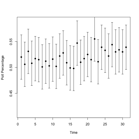
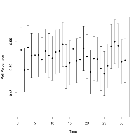
Here are polling percentages from the two types of urns over a one month period.


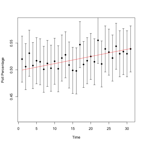
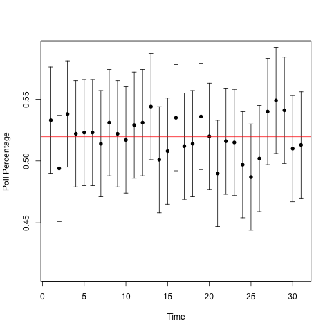
Can you guess which one has the changing urn? It's not obvious. I'll add a line showing the proportion of blue balls in the urn over time to guide the eye.


So the one on the top had the trend: over the 31 days, the proportion of blue balls in the urn went from 50% to 54%. That's a pretty big 'swing' in the population. But we see lots of little 'swings' in both urns, and those are a natural part of the variability from only sampling a fraction of the voting population. (1000 people is a lot less than 126838980.) Those 'swings,' the ones that CNN, Fox News, and MSNBC report on, don't tell us anything. In Silver's homage to the signal processing community, they're noise, not signal.
One more thing to say about the plots before I finish, since they make a very nice demonstration of an basic stats idea that many people mangle, namely, confidence intervals6. The 'error bars' in these plots are 95% confidence intervals for the proportion of blue balls in the urn. In fact, I constructed the confidence intervals using Hoeffding's inequality. I imagine most polling agencies construct their confidence intervals using the asymptotic normality of the proportion estimator. (Because in addition to being the obvious way to estimate a proportion from a random sample, it's also the Maximum Likelihood Estimator for the proportion). For a sample size of 1000, the two methods give you basically the same result.
Let's see how the National Council on Public Polls tells us we should interpret the confidence intervals:
Thus, for example, a "3 percentage point margin of error" in a national poll means that if the attempt were made to interview every adult in the nation with the same questions in the same way at the same time as the poll was taken, the poll's answers would fall within plus or minus 3 percentage points of the complete count's results 95% of the time.
That's a valid interpretation. But I'll let Larry Wasserman's explain a better one, from his All of Statistics:
Some texts interpret confidence intervals as follows: if I repeat the experiment over and over, the interval will contain the parameter 95 percent of the time. This is correct but useless since we rarely repeat the same experiment over and over. A better interpretation is this:
On day 1, you collect data and construct a 95 percent confidence interval for a parameter \(\theta_{1}\). On day 2, you collect new data and construct a 95 percent confidence interval for an unrelated parameter \(\theta_{2}\). On day 3, you collect new data and construct a 95 percent confidence interval for an unrelated parameter \(\theta_{3}\). You continue this way constructing confidence intervals for a sequence of unrelated parameters \(\theta_{1}, \theta_{2}, \theta_{3}, \ldots\) Then 95 percent of your intervals will trap the true parameter value. There is no need to introduce the idea of repeating the same experiment over and over.
Remember, when we're doing frequentist statistics, we care about the frequency properties of the methods we use. A 95 percent confidence interval is a statement about how confident we are in the procedure that we're using, not about our confidence on any given time that we use that procedure. For this particular case, if we look at the second set of plots, our confidence interval should capture the red lines about 95 percent of the time. We see that this time around, we got lucky and captured the true population value every time. Also notice that the confidence intervals for the changing urn still worked. This is why the interpretation of "[asking] the same questions in the same way at the same time as the poll was taken" is useless. We don't need to be doing that for our confidence intervals to work!
I doubt we'll see a day when newscasters begin the polling segments of their coverage with, "Well, nothing all that significant has happened in the polls today, so instead lets throw it over to this video of kittens." But we can hope.
For example, Gallup does one per day.↩
Coming from a 'swing state,' I hear a lot about the mythical undecided voter.↩
Yes, I do know what the electoral college is. And yes, I do realize that the US president isn't determined by the popular vote. But pretending otherwise makes the analysis significantly simpler.↩
I really have to doubt that they know these numbers down to the single digits. But let's pretend.↩
I'm also pretending we only have two types of balls in the urn. Because, let's be honest, we live with a two party system.↩
I would guess that \(P\)-values and confidence intervals are two of the most misunderstood ideas in frequentist statistics.↩