Being as Random as Possible — The Poisson Process
We have to be careful about what we mean when we say something occurs 'at random.' There are many different flavors of random. Basically a distribution for any kind of occasion.
Usually, when we talk about events occurring 'at random,' we have in mind either a Poisson process or a Bernoulli process, depending on if we intend for the events to occur in discrete or continuous time. These processes are two sides of the same coin (bad pun!), and share many of the same properties.
To be slightly more formal, a (homogeneous) Poisson process is a counting process \(N(t)\) that tabulates the number of occurrences of some event in the interval \((0, t]\). We can define the process in terms of its interarrival times (the times between two adjacent events), which must be independent and identically distributed according to an exponential distribution with parameter rate \(\lambda\). We can also define the process in terms of the number of events occurring in some interval \((t_{1}, t_{2}]\), which should be Poisson1 with rate parameter \((t_{2} - t_{1})\lambda\), with the number of occurrences in disjoint intervals should be independent. It takes some thinking to convince oneself that this is mostly what we mean when we say 'at random.' But it does fit the bill. (For example, the Poisson process is memoryless.)
I first started playing around with Poisson processes (computationally) after reading this article about mass shootings over at Empirical Zeal. The article asks the question: are mass shootings really random events? It was written soon after the shooting at Sandy Hook Elementary School, and used a dataset from Mother Jones to put this hypothesis to the test.
Of course, what Aatish has in mind (and what he uses for his hypothesis test) is a Poisson process. (Though, in actuality, he's considering a Bernoulli process, since we only care what day a shooting happens on, which is entirely discrete.) He comes to the more-or-less weak conclusion that the shootings are occurring at random. I had originally planned to do my own analysis of the data. And then research happened.
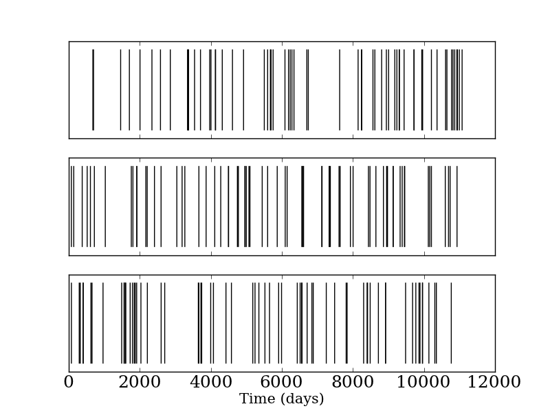
But one thing I did do, which I think is illustrative, is to plot the occurrences of the shootings over time. That is, we want to visualize the point process over time:

Each vertical bar corresponds to the occurrence of an event (in this case, a mass shooting). The top plot is the true occurrences of mass shootings in the US, as reported by Mother Jones. The next two plots are realizations from a Bernoulli process with a rate parameter \(\lambda\) given by the empirical rate from the data (0.006 shootings per day). It's very hard (I think) to distinguish these three data sets, even though the first one corresponds to actual events and the last two correspond to realizations from a Bernoulli process. We see the same sort of 'clumpiness' in both, which is usually what a layperson would use to argue for the shootings being non-random.
Of course, a homogeneous Poisson process is probably a relatively poor model for shootings over time2. We might still want the events to occur 'at random,' but also allow for the rate \(\lambda\) to change over time as well. That is, now we'll let the rate be a function of time, \(\lambda(t)\). This requires some changes to our definition of the Poisson process. Now we have to introduce an integrated rate, \[ \Lambda(t) = \int_{0}^{t} \lambda(\tau) \, d\tau.\] Using the integrated rate, we recover basically the same definition by requiring that the number of events in the interval \((t_{1}, t_{2}]\) be Poisson with rate parameter \(\Lambda(t_{2}) - \Lambda(t_{1})\), and that the number of occurrences in disjoint intervals are still independent. It's not hard to convince yourself that if we take \(\lambda(t) \equiv \lambda\), we recover the same definition as before.
It turns out that inhomogeneous Poisson processes are relatively easy to simulate, using a method called thinning. The method is so-named because we first simulate from a homogeneous Poisson process with rate parameter \(\lambda^{*}\) (which one can do simply by generating the interarrival times according to an exponential distribution with parameter \(\lambda^{*}\)), and then thinning those draws in an intelligent way. For this to make any sense, we need to require that \(\lambda^{*} \geq \lambda(t)\) for all values of \(t\)3.
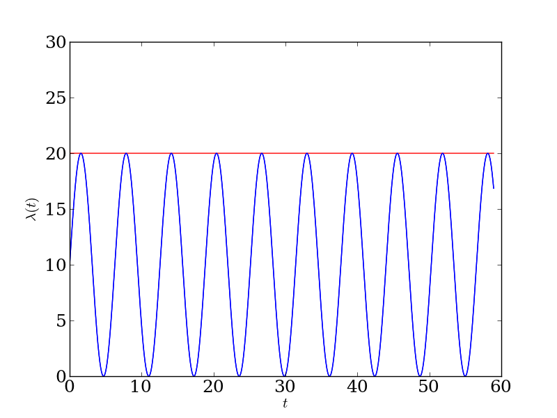
For example, let's take \(\lambda(t) = 10 \sin(t) + 10.\) We need to take \(\lambda^{*} \geq 20\), so let's be judicious and take \(\lambda^{*} = 20\). Here are the two rate functions, the blue one corresponding to the inhomogeneous Poisson process we'd like to simulate from and the red one corresponding to the homogeneous Poisson process we will simulate from and then thin:

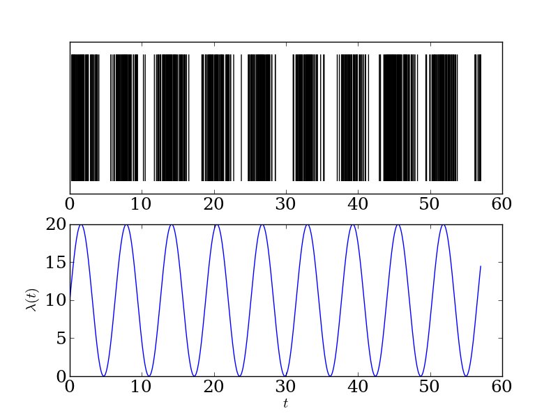
Now it's easy enough to simulate from the Poisson process4, and we get the sort of behavior we'd expect:

This 'bursting' kind of behavior is very reminiscent of the spiking of neurons. In fact, the Poisson process is a favorite model of neurons for theoretical neuroscientists, more because it's tractable than because it's realistic.
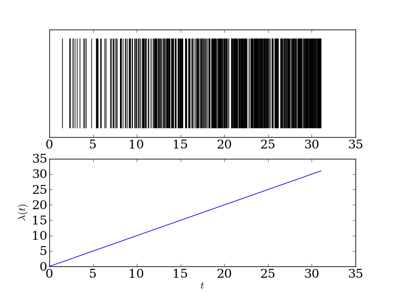
We can also take a rate that ramps up linearly over time, giving us the following behavior:

If we wanted to (which we may), we could even couple together a bunch of inhomogeneous Poisson processes, making the rate of each process dependent on its neighbors. I first read about such a model in this paper by Greg Ver Steeg and Aram Galstyan. You can start to build up very complicated dynamics by coupling together a bunch of 'random' components.
I'm also interested in thinking about how the inhomogeneous Poisson process relates to the inhomogeneous Bernoulli process. The latter would be like flipping a coin, but where the probability of heads possibly changes on each coin flip. The Ver Steeg / Galstyan idea then becomes to look at how coupled coins (where the behavior of a coin depends on the recent behavior of previous coins) behave. This is clearly related to one of my favorite avenues of study, and could make a useful model for the behavior of users on social media.
Hence the name.↩
I just realized that the shooting rate in my neighborhood is only slightly worse than the national average, 0.002 per day. Admittedly, the two shootings in the past three years weren't mass shootings by any means. The real interesting part is their spatial (rather than temporal) locations.↩
We don't need \(\lambda^{*}\) to be constant, actually. We can take it to be piecewise constant, and things work out basically the same. This is important, since if we take \(\lambda^{*}\) to be too big (i.e. the rate of occurrences for the homogeneous process is much higher than the rate for the inhomogeneous process we would like to simulate from), we'll waste a lot of effort simulating occurrences that we'll ultimately throw away.↩
I borrowed the algorithm from Random Number Generation and Monte Carlo Methods by Gentle.↩