Analyzing and Bootstrapping Our Way to a Better Entropy Estimator — Part II, Computational
Before we talk about using bootstrapping to improve our entropy estimator, we need to know what bootstrapping is. For the gory (and very interesting) details, see Larry Wasserman's excellent two part series on the topic on his blog. I'll attempt to give a slightly looser explanation that should provide enough of a background to make the entropy estimator comprehensible.
The idea behind the bootstrap is very simple. We have a data set, call it \(X_{1}, \ldots, X_{n}\), where we assume that each data point in our data set is sampled independently and identically from some underlying distribution \(F\). We're interested in some property of the distribution (its mean, median, variance, quantiles, etc.), call this \(\theta(F)\), but we don't know the distribution and all we have are the data. In this case, we can try to construct an estimator of the property, call this \(\hat{\theta}(X_{1}, \ldots, X_{n} ; F)\), which is now a random variable (since its a function of our data and our data is random). Any time we have a random variable, we would ideally like to talk about its distribution (the 'sampling distribution'), but at the very least we want to know something about its moments.
Bootstrapping allows us to do both, using only the data at hand1. The basic insight is that if we have enough data and compute the empirical cumulative distribution function \[\hat{F}_{n}(x) = \frac{1}{n}\sum_{i = 1}^{n} I[X_{i} \leq x]\] and \(\hat{F}\) is 'close enough'2 to \(F\), then sampling using \(\hat{F}\) is very similar to sampling using \(F\). In this case, we can fall back on simulation based methods ('Monte Carlo methods') typically used when we have a model in mind, but instead of assuming a model a priori, our model is the data. That is, our model is \(\hat{F}\). So we can generate \(B\) new samples from \(\hat{F}\), \[ \{ (X_{1}^{b}, \ldots, X_{n}^{b}) \}_{b = 1}^{B}\] and use these to make probability statements about estimators. For example, if we use each of these samples to get new estimators \(\hat{\theta}^{b} = \hat{\theta}(X_{1}^{b}, \ldots, X_{n}^{b} ; \hat{F})\), its as if we sampled these estimators directly from the underlying distribution \(F\). 'As if' because we didn't sample from \(F\), we sampled from \(\hat{F}\). But if the sample is large enough, then this doesn't matter.
This method was developed by Brad Efron, one of the heavy hitters in modern statistics. It made Larry Wassermnan's list of statistical methods with an appreciable gap between their invention and their theoretical justification (the bootstrap was invented in the 1970s and rigorously justified in some generality in the 1990s). Brad Efron and Rob Tibsharani have an entire book on the subject.
I think that's enough background to bring us to the paper of interest, Bootstrap Methods for the Empirical Study of Decision-Making and Information Flows in Social Systems by Simon DeDeo, Robert Hawkins, Sara Klingenstein and Tim Hitchcock. Throughout, I'll refer to all of the authors as DeDeo, since I've seen Simon speak and he's technically the corresponding author for the paper. Their paper makes no reference to Efron and Tibsharani's book3. Interestingly, the idea of using sampling to estimate the bias of entropy estimators isn't all that new: previous researchers (apparently largely unpublished) suggested using the jackknife (a sampling method very similar to the bootstrap) to estimate bias. See page 1198 of Paniniski's entropy estimation review for the related estimator. DeDeo's paper makes no mention of this estimator either. The silence on these topics is understandable, especially considering DeDeo's massive goal of bringing statistical literacy to the social sciences.
Based on the 'preamble' to this post, the idea behind the bootstrapped bias estimator should be clear. We have our plug-in estimator of entropy, \[ \hat{H} = H(\hat{\mathbf{p}}) = -\sum_{j = 1}^{d} \hat{p}_{j} \log \hat{p}_{j},\] where the \(\hat{p}_{j}\) are just the proportions from our sample \(X_{1}, \ldots, X_{n}\). Since we're dealing with a discrete distribution, \(\hat{\mathbf{p}}\) essentially gives us \(\hat{F}\) (after a few cumulative sums), and we're all set to generate our bootstrap estimates of the bias of \(\hat{H}\). To do this, we pretend that \(\hat{\mathbf{p}}\) is the true distribution, and create \(B\) samples of size \(n\) from the empirical distribution. We then compute the entropy estimate for each bootstrap sample, call these \(\hat{H}^{b}\). Remembering that if we did this procedure using \(\mathbf{p}\) instead of \(\hat{\mathbf{p}}\) that our estimate of the distribution of \(\hat{H}\) would be exact (up to sampling), and we would estimate the bias as \[ \text{Bias}(\hat{H}) = E[\hat{H}] - H(\mathbf{p}) \approx \frac{1}{B} \sum_{b = 1}^{B} \hat{H}^{b} - H(\mathbf{p}),\] since by a Law of Large Numbers argument, the sample average will converge to the true expectation. For bootstrapping, we don't know \(\mathbf{p}\), so we sample the \(\hat{H}^{b}\) using \(\hat{\mathbf{p}}\) instead, and get \[ \widehat{\text{Bias}}(\hat{H}) = E_{\hat{p}}[\hat{H}] - H(\mathbf{\hat{p}}) \approx \frac{1}{B} \sum_{b = 1}^{B} \hat{H}^{b} - H(\hat{\mathbf{p}})\] as our bias estimate. If the gods of statistics are kind, this will be a reasonable estimate of the bias. Since we want the bias to be zero, we subtract this off from our estimator, giving a new estimator \[ \hat{H}_{\text{bootstrap}} = \hat{H} - \left(\frac{1}{B} \sum_{b = 1}^{B} \hat{H}^{b} - H(\hat{\mathbf{p}})\right) = 2 \hat{H} - \frac{1}{B} \sum_{b = 1}^{B} \hat{H}^{b}.\] And thus, with a great deal of computing going on in the background, we have a new way to estimate entropy.
The symbols are nice, but as is usually the case, a picture helps to build intuition. Instead of going through a lot of effort to make my own figure, I stole Figure 1 from DeDeo's paper (see page 2249)4:
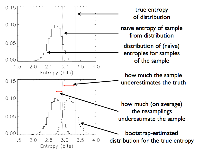
The solid vertical line is the true entropy, what I've been calling \(H(\mathbf{p})\). The dashed line is the plug-in estimate of the entropy, \(\hat{H} = H(\hat{\mathbf{p}})\). The histogram in the top panel is the estimated distribution using the bootstrap samples \(\{ \hat{H}^{b}\}_{b = 1}^{B}\). How far away the average of this distribution is from the estimated entropy gives us a guess at how far our estimated entropy is from the true entropy. Sometimes it seems like turtles all of the way down, but in reality this technique works.
DeDeo, et al., have a Python package that implements their bootstrapped entropy estimator, amongst others. They called it THOTH. From DeDeo's site: "THOTH is named, playfully, after the Ancient Egyptian deity. Thoth was credited with the invention of symbolic representation, and his tasks included judgement, arbitration, and decision-making among both mortals and gods, making him a particularly appropriate namesake for the study of information in both the natural and social worlds."
There's still no final word on the appropriate way to estimate entropy. We've seen three: the maximum likelihood estimator, the Miller-Madow estimator, and the bootstrap estimator. Each of them have their strengths and weaknesses, and will work or fail in different situations.
As a final aside, this has not been a purely academic5 exercise for me. I've been performing mutual information and informational coherence estimation for joint distributions with very large alphabets in the hopes of detecting dynamical and computational communities in social networks6. In these cases, it becomes important to deal with the biases inherent in estimating entropies, since with limited sample sizes, the biases in these estimators seem to indicate much higher mutual information / informational coherence than is actually present. This is bad when you're trying to define functional communities.
Just another example of how careful we have to be when dealing with information theoretic analyses.
Which explains the name 'bootstrap,' at least if you're familiar with early 20th century turns of phrase: we've managed to answer our question (what is the sampling distribution of our estimator) without any extra help.↩
And by the Glivenko-Cantelli Theorem (aka. the Fundamental Theorem of Statistics), it almost surely will.↩
Which is unfortunate, because on page 130 of An Introduction to the Bootstrap, Brad and Rob give a very simple twist on the bootstrap estimator of bias which gives much better convergence results. I'm not completely sure the twist applies to the case DeDeo considers (since typically Brad and Rob are concerned with data from a continuous distribution where data points will never repeat), but if it does, then the change to DeDeo's code should be trivial. Something to look into.↩
Which, to be honest, I didn't fully grasp at my first pass. Without the math, it's hard to get the bootstrapping entropy idea across. Hopefully with the combination of the two, things make a little more sense.↩
Well, depending on ones definition of academic.↩
This will all hopefully show up in a paper in the near to medium future.↩