Simulating Randomness
I've just started watching the lectures of Jim Crutchfield for his course Natural Computation and Self-Organization at UC Davis. These lectures are the closest thing to a textbook for the discipline of computational mechanics, and I need to brush up on some details before my preliminary oral exam sometime this summer.
During the first lecture for the second half of the course (it's broken up into 'Winter' and 'Spring' halves), Jim points out that nature finds uses for randomness. This immediately reminded me of my recent post where I found a (trivial) use for randomness in a simple rock-paper-scissors game. In his lecture, Jim also pointed out that we now know simple ways of generating pseudo-random numbers using deterministic processes. Namely, chaos.
This immediately sent me down a rabbit hole involving the logistic map, everyone's favorite example of a one-dimensional map that, for certain parameter values, can give rise to chaos. For the uninitiated, here's the map:
\[ x_{n+1} = r x_{n}( 1 - x_{n}) \]
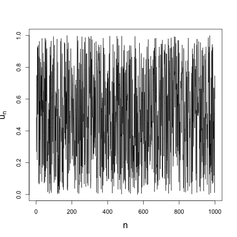
where \(r\) is a positive parameter. This very simple discrete map (it's only a first-order nonlinear difference equation, after all) can lead to chaotic dynamics for values of \(r\) greater than some critical value \(r_{c}\)1. And chaotic systems can look random, at least random enough for most purposes, if you don't know their governing equations. For example, here's 1000 iterations from the logistic map when \(r = 4\):
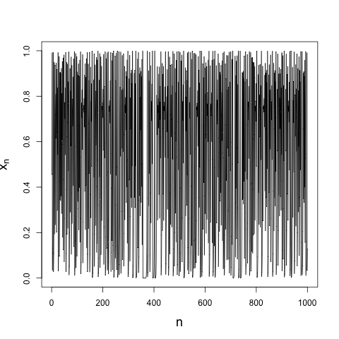
That looks pretty random. Of course, if you were to rerun my code, using exactly the same initial condition I did, you would get exactly the same iterates. It is deterministic, after all.
Which brings me back to Jim's point about nature finding ways to harness chaotic systems to generate pseudo-randomness. Developing one's own pseudo-random number generator can be a fool's errand2, but if you can get something that generates numbers that look like independent draws from a distribution uniform on the interval from 0 to 1, then you're off to the races. These sorts of samples are the building blocks for methods that sample from more interesting distributions, methods like Metropolis-Hastings and Gibbs sampling.
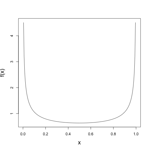
Fortunately, mathematicians far smarter than I (Ulam and von Neumann come to mind) have figured out some properties about the logistic map when \(r = 4\) that I can use to my advantage. For one thing, the natural measure of the logistic map has a density given by \[ f(x) = \left \{ \begin{array}{ll} \frac{1}{\pi \sqrt{x(1-x)}} & : x \in [0, 1] \\ 0 & : \text{ otherwise} \end{array}\right .,\] which if we plot on the interval \([0, 1]\) looks like
The meaning of the natural measure for a dynamical system would require a bit more theory than I want to go into here. But here's the intuition that Ed Ott gave in his chaotic dynamics class. Sprinkle a bunch of initial conditions on the interval \([0, 1]\) at random. Of course, when we say 'at random,' we have to specify at random with respect to what probability measure. The natural measure of a dynamical system is the one that, upon iteration of initial conditions sprinkled according to that measure, results in a measure at each future iteration that hasn't changed. You can think of this as specifying a bunch of initial conditions by a histogram, running those initial conditions through the map, and looking at a histogram of the future iterates. Each initial condition will get mapped to a new point. But each new histogram should look the same as the first. In a sense, we can treat each iterate \(x_{n}\) of the map as if it were drawn from a random variable \(X_{n}\) with this invariant measure.
Clearly, the invariant measure isn't uniform on \([0, 1]\). We'll have to do a little bit more work. If we can treat the iterates \(x_{1}, x_{2}, \ldots, x_{n}\) as though they're random draws \(X_{1}, X_{2}, \ldots, X_{n}\) from the distribution with density \(f\), then we have a way to transform them into iterates that look like random draws \(U_{1}, U_{2}, \ldots, U_{n}\) from a distribution uniform on \([0, 1]\). The usual trick is that if \(X\) has (cumulative) distribution function \(F\), then \(U = F(X)\) will be uniform on \([0, 1]\). That is, applying the distribution function that governs a random variable to itself results in a uniform random variable. We can compute the distribution function for the invariant measure in the usual way, \[ \begin{align*} F(x) &= \int_{-\infty}^{x} f(t) \, dt \\ &= \int_{0}^{x} \frac{1}{\pi \sqrt{t(1-t)}} \, dt \end{align*}.\] After a few trig substitutions, you can work out that the distribution function is given by \[ F(x) = \left \{ \begin{array}{ll} 0 & : x < 0 \\ \frac{1}{2} + \frac{1}{\pi} \arcsin(2x - 1) & : 0 \leq x \leq 1 \\ 1 & : x > 1 \end{array}\right . .\]
Plotting this on the interval \([0, 1]\), we get
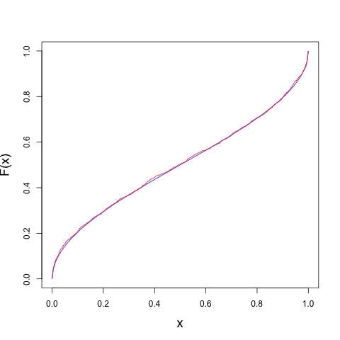
where the blue curve is the true distribution function and the red curve is the empirical distribution function inferred from the thousand iterates. So if we compute \(u_{n} = F(x_{n})\) for each iterate, we should get something that looks uniform. And we do:
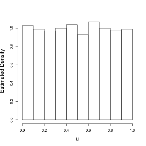
So, the theory works. We've taken a dynamical system that should behave a certain why, and transformed it so that it will look, for the purpose of statistical tests, like draws from a uniform distribution. Here's the transformed iterates:

and a draw of 1000 variates using R's runif3:
Both look pretty random. But there's a fatal flaw in this procedure that would make any cryptoanalyst blush. Remember that the iterates were generated using the map \[ x_{n+1} = r x_{n}( 1 - x_{n}).\] This means that there is a deterministic relationship between each pair of iterates of the map. That is, \(x_{n+1} = M(x_{n})\). We've applied \(F\) to the data, but \(F\) is a one-to-one mapping, and so we also have \(u_{n + 1} = F(M(x_{n})) = H(u_{n})\). In short, if we plot \(u_{n}\) vs. \(u_{n + 1}\) for \(n = 1, \ldots, 999\), we should get something that falls on the curve defined by \(H\). And we do:
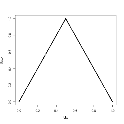
If the iterates were truly random draws from the uniform distribution, they should be spread out evenly over the unit square \([0, 1] \times [0,1]\). Oops. Instead, we see that they look like iterates from another simple dynamical system, the tent map. This is no coincidence. When \(r = 4\), iterates from the tent map and the logistic map are related by the function \(F\), as we've just seen. They're said to be conjugate.
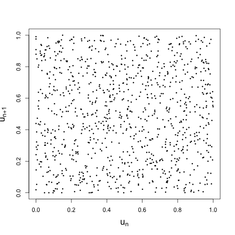
So this is no good, if we want to use these pseudorandom numbers to fool someone. Which got me to thinking: can we combine two deterministic sources to get something that looks random? The process is simple. Generate two sequences of length \(n\) using the logistic map with different initial conditions. Call these \(x_{1}^{(1)}, \ldots, x_{n}^{(1)}\) and \(x_{1}^{(2)}, \ldots, x_{n}^{(2)}\). Map both sequences through \(F\), giving two draws \(u_{1}^{(1)}, \ldots, u_{n}^{(1)}\) and \(u_{1}^{(2)}, \ldots, u_{n}^{(2)}\) that look, except for the recurrence relation above, like random draws from a uniform distribution. Now sort the second sequence from smallest to largest, keeping track of the indices, and use those sorted indices to shuffle the first sequence. That is, compute the order statistics \(u_{(1)}^{(2)}, \ldots, u_{(n)}^{(2)}\) from the second sequence (where those order statistics will still look random, despite the recurrence relation), and use those to wash out the recurrence relationship in the first sequence. If we plot these iterates against each other, as before, we get what we would hope:
Of course, I still wouldn't recommend that you use this approach to generate pseudorandom numbers. And I imagine that other methods (like the Mersenne Twister referenced in the footnotes) are much more efficient. But it is nice to know that, if stranded on a desert island and in need of some pseudorandom numbers, I could generate some on the fly.
What else would I do with all that time?
The term 'chaos' means two very different things to specialists and the general public. I'll point you to a post I made on Quora that gives my working definition.↩
To quote the professor from my first year scientific computing course: "Pseudo-random number generators for the uniform distribution are easy to write but it is very, very difficult to write a good one. Conclusion: don't try to write your own unless you have a month to devote to it."↩
R, Python, and MATLAB (the three major scripting languages used in scientific computing) use a much more sophisticated algorithm called the Mersenne Twister. We'll see why we need something more sophisticated in a moment.↩