Non-Monotonic Transformations of Random Variables
Every school child learns that if you have a random variable \(X\) with probability density function \(f_{X}(x)\), and you transform \(X\) with a monotone function \(g\) to get \(Y = g(X)\), then the density of \(Y\) is given by \[ f_{Y}(y) = \frac{f_{X}(x)}{|g'(x)|} \bigg |_{x = g^{-1}(y)}.\] We need caveats about \(g'(x)\) not being equal to zero, etc. This is standard fair in any elementary probability theory textbook. You can get this result by considering the cumulative distribution function of \(Y\), \(F_{Y}(y) = P(Y \leq y)\), substituting in \(Y = g(X)\), inverting \(g\) (which we can do because it is monotonic), and then remembering that the density of a continuous random variable is the derivative of its cumulative distribution function. (You'll also have to remember the Inverse Function Theorem).
This is useful, but what if \(g\) isn't monotonic? Pedagogically, this is handled by considering the case \(Y = X^2\), and working through what the cumulative distribution function (and thus density) must be. But there is a closed form expression for the density resulting from a general non-monotonic transformation \(g\). For posterity1, here it is:
Let \(X\) be a continuous random variable with density \(f_{X}(x)\), and let \(g\) be a (not necessarily monotonic) transformation. Consider \(Y\), the transformation of \(X\) by \(g\), \(Y = g(X)\). Then the density of \(f_{Y}(y)\) is given by \[ f_{Y}(y) = \sum_{x \in g^{-1}(y)} \frac{f_{X}(x)}{|g'(x)|}.\]
The notation \(x \in g^{-1}(y)\) needs a little explanation, since I didn't assume that \(g\) is monotonic (and thus it need not be invertible). I am considering \(g^{-1}(y)\) as a set, and thus \[ g^{-1}(y) = \{ x : g(x) = y\}.\] For example, if \(g(x) = x^2\), then \(g^{-1}(1) = \{ -1, +1\}\). Thus, for a fixed \(y_{0}\), we have to find all roots to the equation \[ y_{0} = g(x) \ \ \ \ \ \ (*)\] and these will be the elements of our set \(g^{-1}(y_{0})\). It isn't immediately obvious that this is a function of \(y\). But remember that each \(x\) is really a function of \(y\). Once we've fixed a \(y\), we find the \(x\)s that are roots to \((*)\), and thus they must also depend on \(y\).
There you have it. Not quite as nice as the transformation theorem for a monotonic function, but not too much more complicated. The main annoyance is that for each \(y\) we have to find roots of \(y = g(x)\), which need not be a pleasant experience. If we assume that \(g\) is polynomial, things get much better. For example, we could use roots from Python's numerical numpy library. If \(g\) isn't a polynomial, we'll not only have to work a lot harder to find the roots of \(y = g(x)\), but we'll also have to work hard to make sure we've found all of the roots of \(y = g(x)\).
Let's do a polynomial example. Take \(g(x) = x (0.5 - x) (1 - x)\), shown below:
Now let's take \(X\) to be distributed uniformly on \([0, 1]\). Then \(Y = g(X)\) will clearly have support between \([-0.048, 0.048]\) (look at the figure above), and in fact will look like
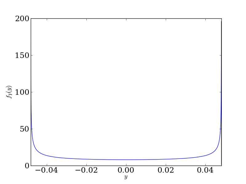
We see that the density goes to infinity at \(y = \pm 0.048\). This is because these are the critical points of \(g(x)\) (again, look at the figure above), so the \(g'(x)\) term in the denominator of our transformation relationship will be zero, putting a singularity at these points. That's fine: the density will still integrate to 1 and all is well in the world.
Now let's use the same theorem, but take \(X\) to be Normal\((0, 1)\). Now \(Y = g(X)\) will have support on the entire real line (since the range of g(x) is the entire real line), and will look like
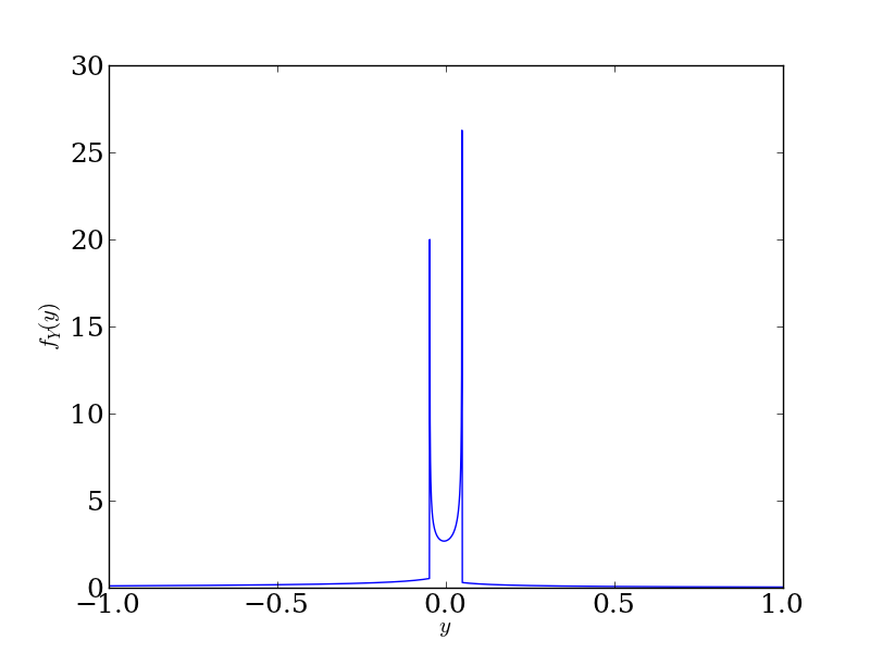
Again, we see that the density goes to infinity at \(y = \pm 0.048\), for the same reason. Also notice the asymmetry since we didn't center \(g(x)\) at 0.
Last, let's do a sanity check by sampling. If we generate a random sample \(X_{1}, \ldots, X_{n}\) according to the distribution of \(X\), and then consider \(Y_{1} = g(X_{1}), \ldots, Y_{n} = g(X_{n})\), the transformed sample \(Y_{1}, \ldots, Y_{n}\) will be distributed according to \(Y\), and we can use a density estimate of \(Y\) from this random sample to get a guess at what \(f_{Y}(y)\) looks like. Let's use histograms:
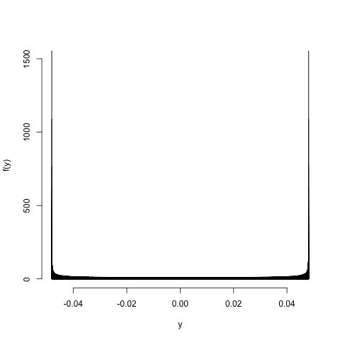
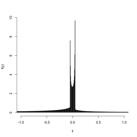
Things work out, as they should. But the singularities at \(y = \pm 0.048\) are less obvious.
Why care about any of this transformation stuff? It shows up in dynamical systems, when we have some map \(M : \mathcal{X} \to \mathcal{X}\) that takes us from a phase space \(\mathcal{X}\) back into itself. We can ask how \(M\) acts on a point \(x_{n}\) by considering \(x_{n+1} = M(x_{n})\), which gives us an orbit of that system \(x_{0}, x_{1}, x_{2}, \ldots\). Similarly, we can ask how \(M\) acts on a set \(A_{n}\) by considering \(A_{n+1} = M(A_{n})\) where \(M(A_{n})\) shorthand like before for \[ M(A_{n}) = \{M(x) : x \in A_{n} \}.\] This gives us an orbit of sets, \(A_{0}, A_{1}, A_{2} \ldots\) Finally, we can ask how \(M\) acts on a density \(f_{n}\) to give a new density \(f_{n+1}\). This idea of \(M\) mapping \(f_{n}\) to \(f_{n + 1}\) is given meaning through the transformation theorem, in this context called the Perron-Frobenius operator. We can then ask if this sequence of densities \(f_{0}, f_{1}, f_{2}, \ldots\) ever settles down to some limiting density \(f_{\infty}\). And this gives us nice results we've seen before.
I tried to Google 'non-monotonic transformation of a random variable' a while back and didn't get very far. I came across my first full treatment of this result in Kobayashi, Mark, and Turin's Probability, Random Processes, and Statistical Analysis. I came across my second treatment yesterday, in Lecture 10 of Natural Computation and Self-Organization.↩