Berry-Esseen Deserves More Praise
Everyone knows the Central Limit Theorem1. In the simplest case, the theorem says that for independent draws from a population that is 'sufficiently well-behaved,' the probability statements that you can make about the sample mean converge, in the limit, to the probability statements you can make about a normal random variable with a mean given by the population mean and a variance given by the population variance over \(n\), the number of data points in your sample. In slightly gorier detail, if we have a sample of independent and identically distributed random variables \(X_{1}, \ldots, X_{n}\) with each having mean \(E[X] = \mu < \infty\) and variance \(\text{Var}(X) = \sigma^{2} < \infty\), then \[\frac{1}{n} \sum_{i = 1}^{n} X_{i} \xrightarrow{D} Y \sim N(\mu, \sigma^{2}/n).\]
This is a very nice theorem. It says that no matter what distribution the \(X_{i}\) have, as long as it's not too pathological2, the sample mean can be treated like a normal random variable for probabilistic computations. And in statistics, these are the sorts of statements we'd like to make.
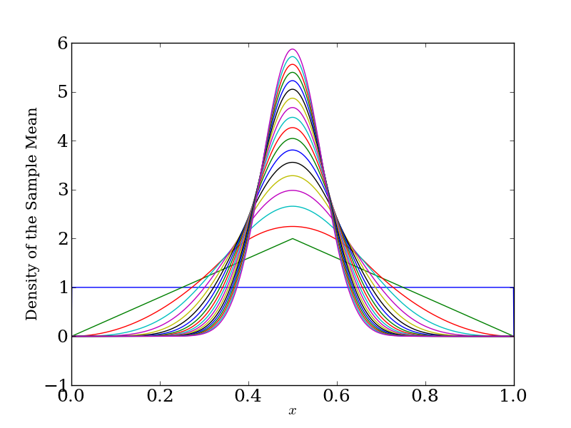
This may seem weird. At least, it seemed weird to me the first time I heard it. What if I take the average of a bunch of Uniform(0, 1) random variables? That is, take a bunch of random variables sampled from the unit step function on \([0, 1]\), and take their average. That starts out decidedly non-normal. But in the limit, you get something that looks3 normal.

The flat curve, horizontal at 1, is the density of a uniform random variable. Each successive curve is the density of \(\bar{X}_{n}\) for larger and larger values of \(n\), going up to 19. As we'd expect, if you average a bunch of numbers between 0 and 1, their average stays between 0 and 1. But we see that, as the central limit theorem promises, the average becomes more and more normal, going from a triangular density at \(n = 2\) to something nearly indistinguishable from a normal density at \(n = 19\). Also as promised, the density becomes more and more concentrated around the true expected value, in this case \(1/2\), as the variance decreases like \(n^{-1/2}\).
This is all standard fair in any introductory statistics course4. What is less standard is the statement about how quickly the sample mean converges to a normal random variable. Asymptotics are nice, but they're, well, asymptotic. Usually we only have a finite amount of data. It would be nice if we could make a statement about how well the \(N(\mu, \sigma^{2}/n)\) approximation works for \(n\) much less than infinity.
And it turns out that we can. The result that gives us the statement is the Berry-Esseen Theorem. Larry Wasserman first brought this result to my attention in his post here. Which, come to think of it, is the first time I saw the theorem stated. I could have sworn I'd also seen it in his All of Statistics, but the theorem isn't in the index.
Without further adieu, here's the theorem.
Theorem: (Berry-Esseen)
Let \(X_{1}, \ldots, X_{n}\) be iid with finite mean \(\mu\) and finite variance \(\sigma^{2}.\) Define
\[Z_{n} = \frac{\sqrt{n} (\bar{X}_{n} - \mu)}{\sigma}\]
Then
\[\sup_{t} |P(Z_{n} \leq t) - \Phi(t)| \leq \frac{0.4784 \beta_{3}}{\sigma^{3} \sqrt{n}},\]
where \(\Phi\) is the standard normal cdf and \(\beta_{3} = E[|X_{i}|^3]\)
There's a lot to chew on here, and it's worth going through the theorem and trying to unpack the consequences for yourself5. But being a bit hand-wavy, it says that if you make a probabilistic statement6 using the normal approximation, for any \(n\) you'll be off at most \(\frac{0.4784 \beta_{3}}{\sigma^{3} \sqrt{n}}\) from if you used the actual sampling distribution of the sample mean for the underlying distribution7. Since we don't usually know the parameters of the true population, let alone the type of distribution, this is a comforting result. Unless the \(\beta_{3}\) term is very large, we won't do so bad in using this approximation: our error goes down like \(n^{-1/2}\). And we can do all sorts of things with this approximation: perform hypothesis tests, construct confidence intervals, you name it.
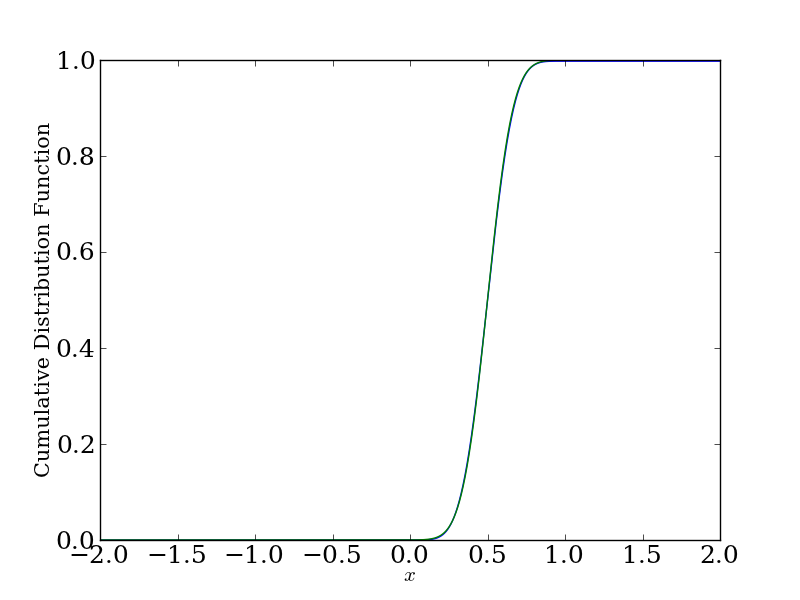
We see from this result that the appropriate way to compare the sampling distribution of the sample mean and the normal approximation is through their cumulative distribution functions. Here's the comparison for \(n = 5\) for the sample mean from a uniform distribution:

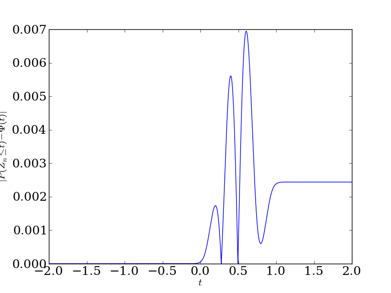
You'll have a hard time telling the difference from this plot, unless you have a really good eye. The help out, here's the absolute error between the true sampling distribution and the normal approximation as a function of \(t\):

We see that even at the worst \(t\), we don't do worse than a difference of 0.007. That's pretty good. Especially considering that the upper bound from the theorem says we'll have error at most 2.20. (We do better than this, which is okay with an upper bound.)
I'll finish with a quote from the book Numerical Recipes8, to remind us what the Central Limit Theorem does and doesn't state, and how people can misunderstand it:
For a hundred years or so, mathematical statisticians have been in love with the fact that the probability distribution of the sum of a very large number of very small random deviations almost always converges to a normal distribution. [...] This infatuation tended to focus interest away from the fact that, for real data, the normal distribution is often rather poorly realized, if it is realized at all. We are often taught, rather casually, that, on average, measurements will fall within +/-\(\sigma\) of the true value 68% of the time, within +/-2\(\sigma\) 95% of the time, and within +/-3\(\sigma\) 99.7% of the time. Extending this, one would expect a measurement to be off by +/-20\(\sigma\) only one time out of \(2 \times 10^{88}\). We all know that "glitches" are much more likely than that!
— W.H. Press et al., Numerical Recipes, Sec. 15.1
I don't know what Press means by 'almost always' (statements like 'almost always' and 'almost surely' mean something very particular in probabilistic contexts). And it sounds like Press had a pretty poor statistics professor, or more likely never took a real course in a statistics department. He makes the mistake I warned against in the footnotes: don't conflate the fact that you can make approximately normal statements about the sample mean with the population being normal. No mathematical statistician thinks that.
That said, here's my response from October 2012:
I don't think it's fair to blame the mathematical statisticians. Any mathematical statistician worth his / her salt knows that the Central Limit Theorem applies to the sample mean of a collection of independent and identically distributed random variables, not to the random variables themselves. This, and the fact that the \(t\)-statistic converges in distribution to the normal distribution as the sample size increases, is the reason we apply any of this normal theory at all.
Press's comment applies more to those who use the statistics blindly, without understanding the underlying theory. Which, admittedly, can be blamed on those same mathematical statisticians who are teaching this very deep theory to undergraduates in an intro statistics class with a lot of (necessary at that level) hand-waving. If the statistics user doesn't understand that a random variable is a measurable function from its sample space to the real line, then he/she is unlikely to appreciate the finer points of the Central Limit Theorem. But that's because mathematical statistics is hard (i.e. requires non-trivial amounts of work to really grasp), not because the mathematical statisticians have done a disservice to science.
Earlier inklings of my railing against the 'statistical-industrial complex.'
Actually, I didn't know Wikipedia has such a nice demonstration of the Central Limit Theorem in action. It puts what I'm about to do to shame.↩
For an example of a 'pathological' random variable, consider the Cauchy distribution. The sum of independent Cauchy random variables is Cauchy, so we have no hope of ever getting a normal random variable out of this limiting process. Oh, and the mean and variance of a Cauchy random variable are not defined.↩
This figure took a surprisingly long time to make. I had to remind myself about convolutions and the Fast Fourier Transform. Fortunately, as they often do, numerics saved me from a lot of tedious integrals.↩
Standard, and yet I imagine very misunderstood. I might be projecting myself onto my students, but I just always had the hunch that they didn't really know what this theorem is saying. For example, here's a common misconception that I might have projected: "The population becomes normal." No, the fact that we don't need that is precisely the power of the Central Limit Theorem.↩
In fact, this sort of 'unpacking' is the type of thing that separates your average undergraduate from your average graduate student. Or, How to Read Mathematics.↩
We make probability statements with cumulative distribution functions, and this is what both \(P(Z_{n} \leq t)\) and \(\Phi(t)\) are, the things we're computing the distance between.↩
Curious about the constant (0.4784)? Read the Wikipedia article to learn about the hard fought struggle to bring it down from its start at 7.59. These battles fascinate me. I wonder if people make careers out of these sorts of results (getting a tighter upper bound), or if most of them are one-off findings in a career spent on other things.↩
This is an interesting book. In graduate school, I've heard two very different perspectives on it. From the mathematicians, especially the numerical analysts, mostly distain. From the physicists, admiration. If the section I quote is any indication of the quality of the rest of the book, I think I'll have to side with the analysts.↩