New Blog, Who Dis?

All future blogging will take place at my GitHub Pages site here.

This blog is kept for posterity and because I occasionally like to look back at the things I once knew.

Yet More on Why R^2 Is Bad, and You Should Feel Bad for Using It

Attention Conservation Notice: A tedious exercise in elementary probability theory showing that $R^{2}$ doesn’t behave the way you think. But you already knew that.

It is a fact universally known that, when the simple linear regression model \[ Y = \beta_{0} + \beta_{1} X + \epsilon\] is correct, the value of $R^{2}$ depends on both:

the variance of the noise term $\epsilon$ and
the variance of the predictor $X$.

The larger the value of $\operatorname{Var}(X)$, the larger the $R^{2}$, even for a fixed noise level. This, to me, is a pretty knock-down argument for why $R^{2}$ is a silly quantity to use for goodness-of-fit, since it only indirectly measures how good a model is, and does little-to-nothing to tell you how well the model fits the data. I even called $R^{2}$ “stupid” in my intro stats class last year, being careful to distinguish between $R^{2}$ being stupid, versus those who use $R^{2}$.

I’m always looking for other examples of how $R^{2}$ behaves counterintuitively, and came across a nice example by John Myles White. He considers a logarithmic regression \[ Y = \log X + \epsilon,\] and demonstrates that for this model, the $R^{2}$ of a linear regression behaves non-monotonically as the variance of the $X$ values increase, first increasing and then decreasing. I wanted to use this to make a Shiny demo showing how $R^{2}$ depends on the variance of the predictor, but stumbled onto a weird “bug”: no matter what value of $\operatorname{Var}(X)$ I chose, I got the same value for $R^{2}$. I eventually figured out why my results differed from White’s, but I will save that punchline for the end. First, a great deal of tedious computations.

Consider the following model for the predictors and the regression function. Let $X \sim U(0, b)$, $\epsilon \sim N(0, \sigma^{2})$, with $X$ and $\epsilon$ independent, and \[ Y = \log X + \epsilon.\] Then the optimal linear predictor of $Y$ is $\widehat{Y} = \beta_{0} + \beta_{1} X$, where \[\begin{align} \beta_{1} &= \operatorname{Cov}(X, Y)/\operatorname{Var}(X) \\ \beta_{0} &= E[Y] - \beta_{1} E[X] \end{align}\] The standard definitions of $R^{2}$ are either as the ratio of the variance of the predicted value of response to the variance of the response: \[ R^{2} = \frac{\operatorname{Var}(\widehat{Y})}{\operatorname{Var}(Y)} = \frac{\beta_{1}^{2} \operatorname{Var}(X)}{\operatorname{Var}(\log X) + \sigma^{2}}\] or as the squared correlation between the predicted value and the response: \[ R^{2} = (\operatorname{Cor}(\widehat{Y}, Y))^{2}.\] For a linear predictor, these two definitions are equivalent.

Because $X$ is uniform on $(0, b)$, $\operatorname{Var}(X) = b^{2}/12$. We compute $\operatorname{Var}(\log X)$ in the usual way, using the “variance shortcut”, as \[ \operatorname{Var}(\log X) = E[(\log X)^{2}] - (E[\log X])^{2}.\] Direct computation shows that \[ E[\log X] = \frac{1}{b} \int_{0}^{b} \log x \, dx = \frac{1}{b} b (\log b - 1) = \log b - 1\] and \[ E[(\log X)^{2}] = \frac{1}{b} \int_{0}^{b} (\log x)^2 \, dx = \frac{1}{b} \cdot (b((\log (b)-2) \log (b)+2)).\] This gives the (perhaps suprising) result that $\operatorname{Var}(\log X) = 1,$ regardless of $b$.

So far, we have that \[ R^{2} = \frac{\beta_{1}^{2} \frac{b^2}{12}}{1 + \sigma^{2}},\] so all that remains is computing $\beta_{1}$ from the covariance of $X$ and $Y$ and the variance of $X$. Using the “covariance shortcut,” \[ \operatorname{Cov}(X, Y) = E[XY] - E[X]E[Y],\] and again via direct computation, we have that \[ E[Y] = E[\log X + \epsilon] = E[\log X] = \log b - 1\] \[ E[X] = \frac{b}{2}\] \[ E[XY] = E[X (\log X + \epsilon)] = E[X \log X] + E[X \epsilon] = E[X \log X] = \frac{2 \, b^{2} \log\left(b\right) - b^{2}}{4 \, b}.\] Overall, this gives us that \[ \operatorname{Cov}(X, Y) = E[XY] - E[X]E[Y] = \frac{1}{4} b \] and thus \[ \beta_{1} = \operatorname{Cov}(X,Y) / \operatorname{Var}(X) = \frac{\frac{1}{4} b}{\frac{b^2}{12}} = \frac{3}{b}\]

Substituting this expression for $\beta_{1}$ into $R^{2}$, we get \[ R^{2} = \frac{3}{4} \frac{1}{1 + \sigma^{2}},\] and thus we see that the $R^{2}$ for the optimal linear predictor, for this model system, only depends on the variance of the noise term.

My model differs from White’s in that his has a predictor that is uniform but bounded away from 0, i.e. $X \sim U(a, b)$ with $a > 0$. Making this choice prevents all of the nice cancellation from occurring (I will spare you the computations), and gives us the non-monotonic depence of $R^{2}$ on $\operatorname{Var}(X)$.

So now we have at least three possible behaviors for $R^{2}$:

$R^{2}$ can increase monotonically with $\operatorname{Var}{X}$, when the linear regression is correct.
$R^{2}$ can increase and then decrease with $\operatorname{Var}{X}$, when White’s model is correct.
$R^{2}$ can remain constant with $\operatorname{Var}{X}$, when the model I chose is correct.

The zoo of possible behaviors for $R^{2}$ hopefully begins to convince you that “getting an $R^{2}$ close to 1 is good!” is far too simple of a story. For our model, we can get an $R^{2}$ of 3/4, in the limit as $\sigma \to 0$, which in some circles would be considered “good,” even though the linear model is clearly wrong for a logarithmic function.

So I’ll stick with calling $R^{2}$ dumb. In fact, I generally avoid teaching it at all, following Wittgenstein’s maxim:

If someone does not believe in fairies, he does not need to teach his children ‘There are no fairies’; he can omit to teach them the word ‘fairy.’

Though I suppose an opposing opinion would be that I should inoculate my students against $R^{2}$’s misuse. But there’s only so much time in a 13 week semester…

Happy Birthday, Ed Lorenz

In honor of Ed Lorenz’s birthday, I want to share a little adventure I took in the nonlinear dynamics literature after finding an error. The error resulted from someone using Wolfram’s MathWorld as a reference for the Kolmogorov-Sinai entropy. I managed to track down the origin of the error (I think) and sent the correction along to MathWorld.

My message to MathWorld is below.

Enjoy!

Error in Kolmogorov Entropy Entry on MathWorld:

The definition you give is not for the Kolmogorov-Sinai / metric entropy. You cite Schuster/Wolfram and Ott. Ott doesn’t contain this definition, so you must be referencing Schuster/Wolfram. Schuster/Wolfram gives this definition on page 96 of their text, citing Farmer 1982a/b. But neither Farmer paper gives this definition for the Kolmogorov-Sinai entropy. Both Farmer 1982a and 1982b give the standard definition, in terms of the supremum of the entropy rate of the symbolized dynamics over all finite partitions of the state space. The best guess I could find for the origin of the Schuster/Wolfram error was in Grassberger 1983, which cites Farmer 1982a, and gives the incorrect definition for the Kolmogorov-Sinai entropy that you provide. Interestingly, the Grassberger paper also gets the page number wrong for Farmer 1982a: citing page 566 rather than 366.

Thanks for the chance to go on this mathematical excavation!

References:

Farmer 1982a: J. Doyne Farmer. "Chaotic attractors of an infinite-dimensional dynamical system." Physica D: Nonlinear Phenomena 4.3 (1982): 366-393.

Farmer 1982b: J. Doyne Farmer. "Information dimension and the probabilistic structure of chaos." Zeitschrift für Naturforschung A 37.11 (1982): 1304-1326.

Grassberger 1983: Peter Grassberger, and Itamar Procaccia. "Estimation of the Kolmogorov entropy from a chaotic signal." Physical Review A 28.4 (1983): 2591.

So You Think You Can Statistics: Overlapping Confidence Intervals, Statistical Significance, and Intuition

Attention Conservation Notice: I begin a new series on the use of common sense in statistical reasoning, and where it can go wrong. If you care enough to read this, you probably already know it. And if you don’t already know it, you probably don’t care to read this. Also, I’m cribbing fairly heavily from the Wikipedia article on the t-test, so I’ve almost certainly introduced some errors into the formulas, and you might as well go there first. Also also: others have already published a paper and written a Masters thesis about this.

Suppose you have two independent samples, $X_{1}, \ldots, X_{n}$ and $Y_{1}, \ldots, Y_{m}$. For example, these might be the outcomes in a control group ($X$) and a treatment group ($Y$), or a placebo group and a treatment group, etc. An obvious summary statistic for either sample, especially if you’re interested in mean differences, is the sample mean of each group, $\bar{X}_{n}$ and $\bar{Y}_{m}$. It is then natural to compare the two and ask: can we infer a difference in the averages of the populations from the difference in the sample averages?

If a researcher is clever enough to use confidence intervals rather than P-values, they may begin by constructing confidence intervals for $\mu_{X}$ and $\mu_{Y}$, the (hypothetical) population means of the two samples. For reasonably sized samples that are reasonably unimodal and symmetric, a reasonable confidence interval is based on the $T$-statistic. Everyone learns in their first statistics course that the $1 - \alpha$ confidence intervals for the population means under the model assumptions of the $T$-statistic are

\[I_{\mu_{X}} = \left[\bar{X}_{n} - t_{n - 1, \alpha/2} \frac{s_{X}}{\sqrt{n}}, \bar{X}_{n} + t_{n-1, \alpha/2} \frac{s_{X}}{\sqrt{n}}\right]\]
and
\[I_{\mu_{Y}} = \left[\bar{Y} _{m}- t_{m - 1, \alpha/2} \frac{s_{Y}}{\sqrt{m}}, \bar{Y}_{m} + t_{m - 1, \alpha/2} \frac{s_{Y}}{\sqrt{m}}\right],\]
respectively, where $s_{X}$ and $s_{Y}$ are the sample standard deviations. These are the usual ‘sample mean plus or minus a multiple of the standard error’ confidence intervals. It then seems natural to see if these two intervals overlap to determine whether the population means are different. This sort of heuristic, for example, is described here and here. Yet despite the naturalness of the procedure, it also happens to be incorrect[1].

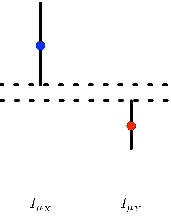
To see this, consider the confidence interval for the difference in the means, which in analogy to the two confidence intervals above I will denote $I_{\mu_{X} - \mu_{Y}}$. If we construct the confidence interval by inverting[2] Welch’s t-test, then our $1 - \alpha$ confidence interval will be

\[I_{\mu_{X} - \mu_{Y}} = \left[ (\bar{X}_{n} - \bar{Y}_{m}) - t_{\nu, \alpha/2} \sqrt{\frac{s_{X}^{2}}{n} + \frac{s_{Y}^{2}}{m}}, \\ (\bar{X}_{n} - \bar{Y}_{m}) + t_{\nu, \alpha/2} \sqrt{\frac{s_{X}^{2}}{n} + \frac{s_{Y}^{2}}{m}} \right]\]

where the degrees of freedom $\nu$ of the $T$-distribution is approximated by

\[\nu \approx \frac{\left(\frac{s_{X}^{2}}{n} + \frac{s_{Y}^{2}}{m}\right)^{2}}{\frac{s_{X}^{4}}{n^{2}(n - 1)} + \frac{s_{Y}^{4}}{m^{2} (m - 1)}}.\]

This is a[3] reasonable confidence interval, where it would be a very good confidence interval if you’re willing to assume that the two populations are exactly normal but have unknown and possibly different standard deviations. This is again a ‘sample mean plus or minus a multiple of a standard error’-style confidence interval. How does it relate to the ‘overlapping confidence intervals’ heuristic?

Well, if we’re only interested in using our confidence intervals to perform a hypothesis test for whether we can reject (using a test of size $\alpha$) that the population means are not equal, then our heuristic says that the event $I_{\mu_{X}} \cap I_{\mu_{Y}} = \varnothing$ (i.e. the individual confidence intervals do not overlap) should be equivalent to $0 \not \in I_{\mu_{X} - \mu_{Y}}$ (i.e. the confidence interval for the difference does not contain $0$).

Well, when does $I_{\mu_{X}} \cap I_{\mu_{Y}} = \varnothing$? Without loss of generality, assume that $\bar{X}_{n} > \bar{Y}_{m}$. In that case, the confidence intervals do not overlap precisely when the lower endpoint of $I_{\mu_{X}}$ is greater than the upper endpoint of $I_{\mu_{Y}}$,

That is,

\[\bar{X}_{n} - t_{n-1, \alpha/2} \frac{s_{X}}{\sqrt{n}} > \bar{Y}_{m} + t_{m - 1, \alpha/2} \frac{s_{Y}}{\sqrt{m}},\]

and rearranging,

\[\bar{X}_{n} - \bar{Y}_{m} > t_{n-1, \alpha/2} \frac{s_{X}}{\sqrt{n}} + t_{m - 1, \alpha/2} \frac{s_{Y}}{\sqrt{m}}. \hspace{1 cm} \mathbf{(*)}\]

And when isn’t 0 in $I_{\mu_{X} - \mu_{Y}}$? Precisely when the lower endpoint of $I_{\mu_{X} - \mu_{Y}}$ is greater than 0, so

\[\bar{X}_{n} - \bar{Y}_{m} - t_{\nu, \alpha/2} \sqrt{\frac{s_{X}^{2}}{n} + \frac{s_{Y}^{2}}{m}} > 0\]

Again, rearranging

\[\bar{X}_{n} - \bar{Y}_{m} > t_{\nu, \alpha/2} \sqrt{\frac{s_{X}^{2}}{n} + \frac{s_{Y}^{2}}{m}}. \hspace{1 cm} \mathbf{(**)}\]

So for the heuristic to ‘work,’ we would want $\mathbf{(*)}$ to imply $\mathbf{(**)}$. We can see a few reasons why this implication need not hold: the $t$-quantiles do not match and therefore cannot be factored out, and even if they did, $\frac{s_{X}}{\sqrt{n}} + \frac{s_{Y}}{\sqrt{m}} \neq \sqrt{\frac{s_{X}^{2}}{n} + \frac{s_{Y}^{2}}{m}}$. We do have that $\frac{s_{X}}{\sqrt{n}} + \frac{s_{Y}}{\sqrt{m}} \geq \sqrt{\frac{s_{X}^{2}}{n} + \frac{s_{Y}^{2}}{m}}$ by the triangle inequality. So if we could assume that all of the $t$-quantiles were equivalent, we could use the heuristic. But we can’t. Things get even more complicated if we use a confidence interval for the difference in the population means based on Student’s $t$-test rather than Welch’s.

As far as I can tell, the triangle inequality argument is the best justification for the non-overlapping confidence intervals heuristic. For example, that is the argument made here and here. But this is based on confidence intervals from a ‘$Z$-test,’ where the quantiles come from a standard normal distribution. Such confidence intervals can be justified asymptotically, since we know that a sample mean standardized by a sample standard deviation will converge (in distribution) to a standard normal by a combination of the Central Limit Theorem and Slutsky’s theorem[4]. Thus, this intuitive approach can give a nearly right answer for large sample sizes in terms of whether we can reject based on overlap. However, you can still have the case where the one sample confidence intervals do overlap and yet the two sample test says to reject. See more here.

My introduction to the overlapping confidence interval heuristic originally arose in the context of this journal article on contrasting network metrics (mean shortest path length and mean local clustering coefficient) between a control group and an Alzheimers group. The key figure is here, and shows a statistically significant separation between the two groups in the Mean Shortest Path Length ($L_{p}$ in their notation, right most figure) at certain values of a thresholded connectivity network. Though, now looking back at the figure caption, I realize that their error bars are not confidence intervals, but rather standard errors[5]. So, we can think of these as 84% confidence intervals for a large enough sample. They will be about half as long as a 95% confidence interval. But even doubling them, we can see a few places where the confidence intervals do not overlap and yet the two sample $t$-test result is not significant.

Left as an exercise for the reader: A coworker asked me, “If the individual confidence intervals don’t tell you whether the difference is (statistically) significant or not, then why do we make all these plots with the two standard errors?” For example, these sorts of plots. Develop an answer that (a) isn’t insulting to non-statisticians and (b) maintains hope for the future of the use of statistics by non-statisticians.

By ‘incorrect,’ here I mean that we can find situations where the heuristic will give non-significance when the analogous two sample test will give significance, and vice versa. To quote Cosma Shalizi, writing in a different context, “The conclusions people reach with such methods may be right and may be wrong, but you basically can’t tell which from their reports, because their methods are unreliable.” ↩
I plan to write a post on this soon, since a quick Google search doesn’t turn up any simple explanations of the procedure for inverting a hypothesis test to get a confidence interval (or vice versa). Until then, see Berger and Casella’s Statistical Inference for more. ↩
A because you can come up with any confidence interval you want for a parameter. But it should have certain nice properties like attaining the nominal confidence level while also being as short as possible. For example, you could take the entire real line as your confidence interval and capture the parameter value 100% of the time. But that’s a mighty long confidence interval. ↩
We don’t get the convergence ‘for free’ from the Central Limit Theorem alone because we are standardizing with the sample, rather than the population, standard deviation. ↩
There is a scene in the second PhD Comics movie where an audience member asks a presenter, “Are your error bars standard deviations or standard errors?” The presenter doesn’t know the answer, and the audience is aghast. After working through this exercise, this joke is both more and less funny. ↩

Good Science

Experimentalists think that a clever experiment will reveal the truth no matter what analysis they perform. ("If your result needs a statistician then you should design a better experiment." - Ernest Rutherford)

Analysts think that a clever analysis will reveal the truth no matter what experiment they perform. ("If the difficulty of a physiological problem is mathematical in essence, then physiologists ignorant of mathematics will get precisely as far as one physiologist ignorant of mathematics, and no further." - Norbert Wiener)

Good science lies somewhere between these two extremes.

All Your Tweets Belong to Us

I spoke today at the AMSC Student Seminar¹ on some of my research related to modeling human behavior in digital environments².

The (slightly censored³) slide deck can be found here.

For any UMD readers out there, the AMSC Student Seminar takes place every other Friday at 10am in CSS 4301. With free food!↩
In fact, the title of the talk was "Computational Models of Human Behavior in Digital Environments." But the title of this post is probably more accurate.↩
If you wanted to see the uncensored version, you had to be at the talk!↩

Counting Fish — Point Processes, the Coefficient of Variation, and the Fano Factor

Errata (21 June 2023): I erroneously stated that the mean and standard deviation of an exponential random variable with rate $\lambda$ are both $\lambda$. They are of course both $1 / \lambda$.

I finally got around to reading Burstiness and Memory in Complex Systems out of Barabási's lab.

This lead me to looking up both the coefficient of variation, which the paper uses as the numerical measure for the burstiness of a point process, and a closely related quantity, the Fano factor. A quick Google search turns up a few hits, but none of them are particularly illuminating compared to the picture I have formed in my head¹.

So here's that picture².

We'll begin with the story about the homogeneous Poisson process. I've already written about it elsewhere, so I won't rehash a lot of the details here. The main thing to know about the Poisson process is that:

It's a counting process. That is, the stochastic process $(N(t))_{t \in \mathbb{R}^{+}}$ takes on values in $\mathbb{N}$, which we can think of as the number of 'counts' of some occurrence from time 0 to time $t$. Think of the number of particles of radiation emitted by an atom, or the number of horse-related deaths in the Prussian army over time.
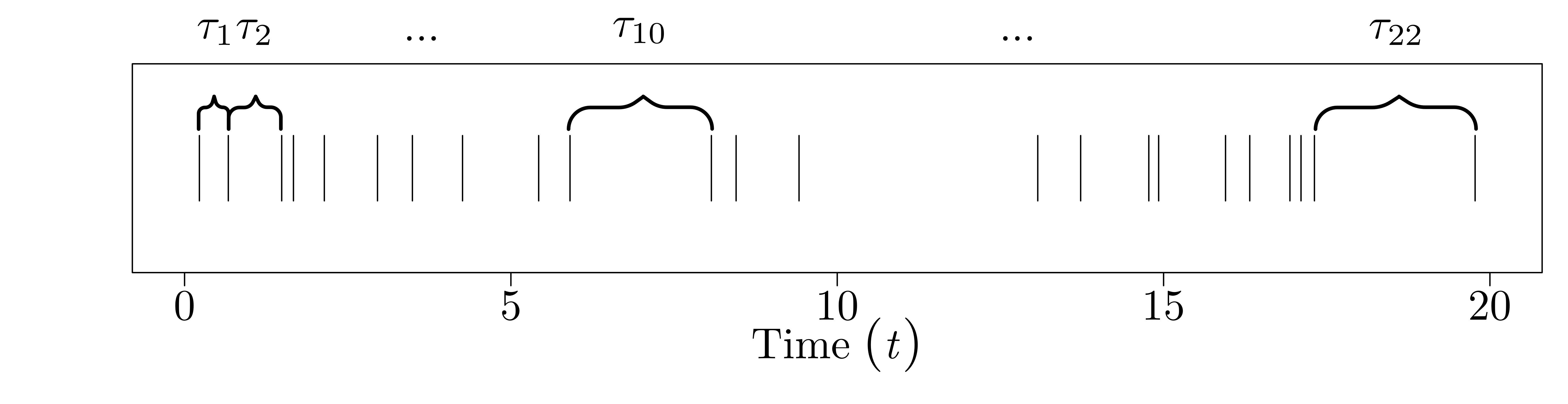
The times at which a count occurs, i.e. those times $t$ when $N(t)$ makes a jump, are themselves random. Let's call those random jump / count times $T_{0}, T_{1}, \ldots, T_{N-1}.$

The picture to have in your head looks something like this:

where the occurrences are on the top, and the count process $N(t)$ is on the bottom. ($N(t)$ should be piecewise constant, since it's defined for all $t \in \mathbb{R}^{+}$. But I'm in a rush.)

Since $T_{i-1}$ and $T_{i}$ are random, so is the time between them, $\tau_{i} = T_{i} - T_{i-1}$. I'll call this the interarrival time (since it's the time between two 'arrivals'). Not only is it random, but for the Poisson process, we define the $\tau_{i}$ to be iid exponential, with rate parameter $\lambda$. That is, $\tau_{0}, \ldots, \tau_{N-1} \stackrel{\text{iid}}{\sim} \text{Exp}(\lambda).$
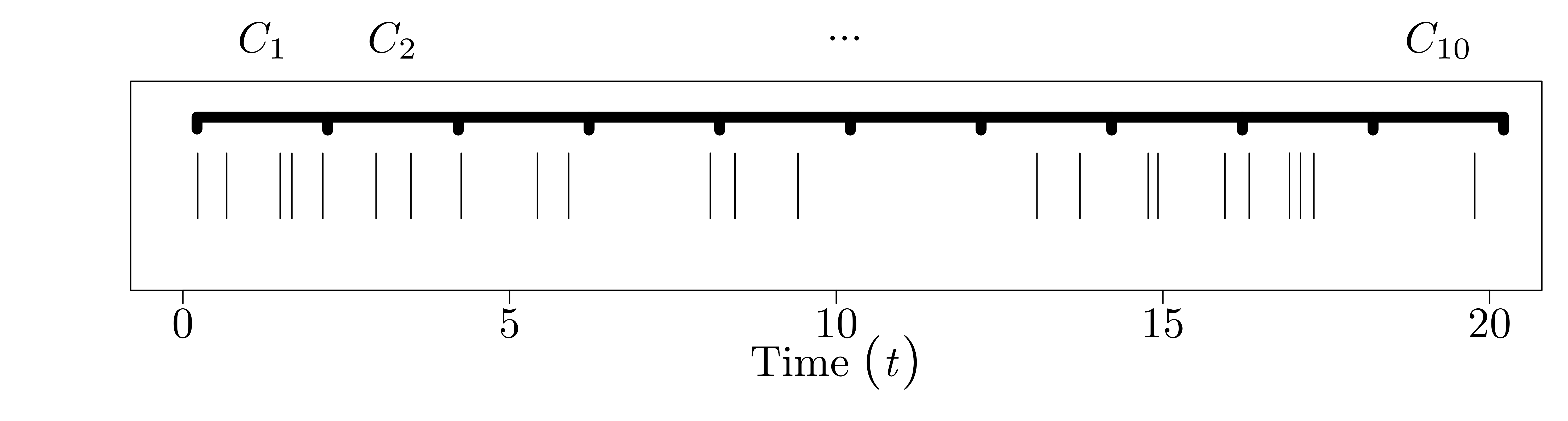
Since the counts occur at random times, the number of counts in a time interval $[(i - 1)\Delta, i \Delta]$ of length $\Delta$ is also random. Call this value $C_{i}$. Again, for the Poisson process, we specify that the number of counts in disjoint intervals of length $\Delta$ are iid Poisson with rate parameter $\Delta \lambda$. That is, $C_{0}, \ldots, C_{N-1} \stackrel{\text{iid}}{\sim} \text{Poisson}(\Delta \lambda).$

The picture for the interarrival times looks like this:

And the picture for the binned counts looks like this:

Now we have everything we need to define the coefficient of variation and the Fano factor, which basically correspond to how 'bursty' the process is from either the interarrival perspective or the count perspective. The coefficient of variation is about the shape of the interarrival time distribution, in particular how its standard deviation relates to its mean: \[\text{CoV} = \frac{\sqrt{\text{Var}(\tau)}}{E[\tau]}.\] Then the Fano factor is about the shape of the binned count distribution, in particular how its variance relates to its mean: \[\text{FF} = \frac{\text{Var}(C)}{E[C]}.\] Both of these ratios measure how 'clumpy' the count process is. For the coefficient of variation, this is direct: if the standard deviation of the interarrival times is much larger than the mean of the interarrival times, this means that we generally expect the occurrence times to be close together ('on average'), but that occasionally we should get large gaps between consecutive occurrences, which is what allows us to define 'bursts.' For the Fano factor, the clumpiness idea works out as so: if the expected number occurrences in a bin is small compared to the variation in the counts in a bin, then we must have a few bins that captured a lot of occurrences, and thus bursts / clumps occurred in those bins.

For a Poisson process, both the coefficient of variation and the Fano factor are 1, since an exponential random variable with rate parameter $\lambda$ has both mean and standard deviation $1 / \lambda$, and a Poisson random variable with rate parameter $\Delta \lambda$ has mean and variance $\Delta \lambda$. This is, of course, a necessary but not sufficient condition for a process to be Poisson. We are only considering the first two moments, after all. For instance, you could construct a non-Poissonian counting process whose interarrival distribution has its mean equal to its standard deviation, while still not being exponential. (Exercise: construct such a process!)

Neither the coefficient of variation nor the Fano factor is particularly mysterious when we stop to clarify what they're actually quantifying. The confusion comes when we forget to distinguish between sample and population values. But that's what 'statisticians do it better.'

The Wikipedia article on the Fano factor was clearly written by a physicist. Which seems appropriate, given that Ugo Fano was a physicist. And not to be confused with Robert Fano, who did a great deal of work in information theory. (Not that I'd ever make that mistake.)↩
I keep using the word 'picture' deliberately. I have convinced myself that mathematicians (and scientists) should, when possible, show rather than tell. I'm reminded of this quote by Richard Feynman: "I had a scheme, which I still use today when somebody is explaining something that I'm trying to understand: I keep making up examples. For instance, the mathematicians would come in with a terrific theorem, and they're all excited. As they're telling me the conditions of the theorem, I construct something which fits all the conditions. You know, you have a set (one ball) - disjoint (two balls). Then the balls turn colors, grow hairs, or whatever, in my head as they put more conditions on. Finally they state the theorem, which is some dumb thing about the ball which isn't true for my hairy green ball thing, so I say, 'False!'"↩

The Lost Art of Hand-made Graphs; Or, The Rise of Mass Produced Charts

I recently read this post by Dr. Drang over at And now it's all this on the lost art of making charts¹. This article reminded me of something that is blindingly obvious in retrospect: until very recently, almost all the portrayals of scientific data were hand-drawn.

Take this graphic of Napoleon's attempted invasion of Russia by Charles Joseph Minard². Or Dr. John Snow's map identifying the locations of cholera outbreaks in London. Both were done by hand, and both are very artful.

And now we have these. And these. And slightly better, these.

Graphics have become industrialized. You can tell whether or not someone is using R, Matlab, Excel, or gnuplot by inspection. Different communities have different standards. But they're definitely no longer done by hand. Sometimes this is good. Sometimes this is bad.

On the opposite end of the spectrum, just thirty odd years ago, everyone had to do mathematical typesetting by hand. And now we have Donald Knuth's gift to the world: LaTeX³. Though that can also make papers like these seem way more legit than they should⁴.

It's interesting to see scientific analysis become more mass produced.

Now these things are called 'infographics' or 'data visualization.' I don't really know what makes those things different from charts.↩
Apparently Minard is considered by some the Father of Infographics.↩
Not to mention his contribution to the world via The Art of Computer Programming.↩
I have to admit that when I read a paper on the arXiv typeset in Microsoft Word, I automatically deduct ten to twenty legitimacy points. I shouldn't, but I do.↩

Paley-Zygmund and Inconsistent Estimators

Cosma Shalizi was kind enough to share a proof that non-vanishing variances implies inconsistent estimators, related to my previous post on spectral density estimators¹. The proof is quite nice, and like many results in mathematical statistics, involves an inequality. Since a cursory Google search doesn't reveal this result, I post it here for future Googlers.

We start by noting the Paley-Zygmund inequality, a 'second moment' counterpart to Markov's inequality:

Theorem: (Paley-Zygmund) Let $X$ be a non-negative random variable with finite mean $m = E[X]$ and variance $v = \text{Var}(X)$. Then for any $a \in (0, 1)$, we have that

\[P(X \geq a m) \geq (1 - a)^{2} \frac{m^{2}}{m^{2} + v}.\]

We're interested in showing: if $\text{Var}\left(\hat{\theta}\right)$ is non-vanishing, then $\hat{\theta}$ is not a consistent estimator of $\theta$. Consistency² of an estimator is another name for convergence in probability. To show convergence in probability, we'd need to show that for all $\epsilon > 0$, \[ P\left(\left|\hat{\theta}_{n} - \theta\right| > \epsilon\right) \xrightarrow{n \to \infty} 0.\] Thus, to show that the estimator isn't consistent, it is sufficient to find a single $\epsilon > 0$ such that we don't converge to 0. To do so, take $X = (\hat{\theta}_{n} - \theta)^{2}$. This is clearly greater than or equal to zero, so we can apply the Zygmund-Paley inequality. Substituting into the inequality, we see \[P\left(\left(\hat{\theta}_{n} - \theta\right)^{2} \geq a m\right) \geq (1 - a)^{2} \frac{m^{2}}{m^{2} + v}\] where \[m = E\left[\left(\hat{\theta}_{n} - \theta\right)^{2}\right] = \text{MSE}\left(\hat{\theta}_{n}\right) = \text{Var}\left(\hat{\theta}_{n}\right) + \left\{ \text{Bias}\left(\hat{\theta}_{n}\right)\right\}^{2}\] and \[ v = \text{Var}\left(\left(\hat{\theta}_{n} - \theta\right)^{2}\right).\] If we assume the estimator is asymptotically unbiased, then $m$ reduces to the variance of $\hat{\theta}_{n}$. Next, we choose a particular value for $a$, say $a = 1/2$. Substituting, \[P\left(\left(\hat{\theta}_{n} - \theta\right)^{2} \geq \frac{1}{2} m\right) \geq \frac{1}{4} \frac{m^{2}}{m^{2} + v}.\] Finally, note that \[ \left\{ \omega : \left(\hat{\theta}_{n} - \theta\right)^{2} \geq \frac{1}{2} m\right\} = \left\{ \omega : \left|\hat{\theta}_{n} - \theta\right| \geq \sqrt{\frac{1}{2} m}\right\}.\]

Let $m'$ be the limiting (non-zero) variance of $\hat{\theta}$. Then for any $\epsilon_{m'}$ we choose such that \[ \epsilon_{m'} \leq \sqrt{\frac{1}{2} m'},\] we see that \[ P\left(\left|\hat{\theta}_{n} - \theta\right| > \epsilon_{m'}\right) \geq P\left(\left(\hat{\theta}_{n} - \theta\right)^{2} \geq \frac{1}{2} m\right) \geq \frac{1}{4} \frac{m^{2}}{m^{2} + v} \geq 0\] and thus \[ P\left(\left|\hat{\theta}_{n} - \theta\right| > \epsilon_{m'}\right) \not\to 0. \] Thus, we have a found an $\epsilon > 0$ such that the probability does not converge to 0, and $\hat{\theta}_{n}$ must be inconsistent.

Which, admittedly, was posted ages ago. I promise I'll post more frequently.↩
Well, weak consistency. Strong consistency is about convergence to the correct answer almost surely. There is also mean-square consistency, which is a form of convergence in quadratic mean. Have I mentioned that good statistics requires a great deal of analysis?↩

Estimating the Power Spectral Density: Part I, The Periodogram, and Why Not to Use It

If you give a physicist, electrical engineer, or applied harmonic analyst a time series (signal), one of the first things they'll do is compute its Fourier transform¹. This is a reasonable enough thing to do: the Fourier transform gives you some idea of the dominant 'frequencies' in the time series, and might give you important information about the large scale structure of the signal. For example, if you compute the Fourier transform of a pure sinusoid, and plot its squared modulus (power spectrum), you'll see a delta function at the frequency of the sinusoid. Similarly, if you compute the power spectrum of the sum of sinusoids, you'll get out a mixture of delta functions, with a delta function at each frequency. This is useful, especially if you signal really is just the sum of sines and cosines: you've reduced the information you have to keep (the entire signal) to a few numbers (the frequencies of the sinusoids).

But sometimes, you don't have any good reason to believe that the time series you are looking at can be decomposed (nicely) into sines and cosines. In fact, the thing you're looking at may be a realization from some stochastic experiment, in which case you know that nice representations of that realization may be hard to come by. In these cases, we can treat the time series as a realization from some stochastic process $\{ X_{t}\} $sampled at $T$ time points, $t = 1, 2, \ldots, T$. That is, we observe $X_{1}, X_{2}, \ldots, X_{T}$ and want to say something meaningful about it. It's still quite natural to take the Fourier transform of the time series and square it with the hope that some structure pops out. Since we have the signal sampled at discrete collection of points, what we're really going to compute is the discrete Fourier transform² of the data, \[ d(\omega_{j}) = n^{-1/2} \sum_{t = 1}^{T} X_{t} e^{-2 \pi \omega_{j} t},\] where $\omega_{j} = \frac{j}{T}$, and $j = 0, 1, 2, \ldots, T - 1$. The discrete Fourier transform is a means to an end, namely the periodogram of the data, \[ I(\omega_{j}) = |d(\omega_{j})|^{2},\] which is the squared modulus of the discrete Fourier transform. The periodogram is the discrete analog to the power spectrum, in the same way that the discrete Fourier transform is the discrete analog to the Fourier transform.

If we were observing a purely deterministic signal, then we'd be done. Ideally, as we collect more and more data from a signal that isn't changing over time, we'll be able to resolve our estimate of the spectral density better and better.

If the signal is stochastic in nature, things are more complicated. It turns out that the periodogram is an unbiased but inconsistent estimator for the spectral density of a stochastic process. In particular³, one can show that asymptotically, at each Fourier frequency $\omega_{j}$, while \[E[I(\omega_{j})] = f(\omega_{j}),\] that is, the estimator is unbiased, it also holds that \[ \text{Var}(I(\omega_{j})) = (f(\omega_{j}))^{2} + O(1/n).\] That is, the variance of the estimator approaches a (possibly non-zero) constant, depending on the true value of the spectral density⁴. In other words, even as you collect more and more data, the variance of your estimator for $f$ at any point will not go down! The estimator remains 'noisy' even in the limit of infinite data!

The way to solve this is to 'share' information at the various $\omega_{j}$ about $f(\omega_{j})$ by smoothing the $I(\omega_{j})$ values. That is, we perform a regression of $I(\omega_{j})$ on $\omega_{j}$ to get a new estimator $J(\omega_{j})$ that will no longer be unbiased (since $f(\omega_{j})$ is generally not equal to $f(\omega_{j} \pm \Delta \omega)$), but can be made to have vanishing variance (since as we collect more and more data, we can 'borrow' from more and more values near $\omega_{j}$ to estimate $f(\omega_{j})$ using $I(\omega_{j}))$. This is the usual bias-variance tradeoff that seems to occur everywhere in statistics: we sacrifice unbiasedness to get reduction in variance in hopes that overall we reduce the mean-squared error of our estimator.

Since this is a regression problem (again, regressing $I(\omega_{j})$ on $\omega_{j}$), we can solve it using any of favorite regression techniques⁵. As I said in the footnote below, Chapter 7 of Nonlinear Time Series by Fan and Yao has a nice survey of various standard (and some more modern) techniques for doing this regression / smoothing. One favorite method, especially for physicists who are hungry to find 1/f noise everywhere, is to fit a line through the periodogram. This is a form of regression / smoothing, but it seems to put the cart before the horse: if you go searching for a line, you'll find it. Then again, there are worse things you could do with a linear regression.

I've added 'inconsistency of the periodogram' to my list of data analysis mistakes not to make in the future. Lesson learned: always smooth your squared DFT!

Postscript: There are other ways to think about why we should smooth the periodogram that ring more true to experimentalists⁶. For some reason, I always find these stories (which ring more true with reality) less appealing than thinking about the problem statistically using a 'generative model' for the signal from the start.

Interestingly, if you give a physicist who specializes in nonlinear dynamics a time series, one of the first things they'll do is compute an embedding.↩
With any Fourier transform-type work, you always have to be careful about the $2 \pi$ terms that show up here, there, and everywhere. I'm following the convention used in Shumway and Stoffer's Time Series Analysis and Its Applications.↩
See, for example, Section 2.4 of Nonlinear Time Series by Fan and Yao, where they give an excellent theoretical treatment of the problems using the raw periodogram, and Chapter 7 of the same text, where they offer up some very nice solutions.↩
This is a point I'm less clear on: if you have an asymptotically unbiased estimator, and its variance goes to zero, then the estimator is consistent (it converges in probability to its true value). You can show this relatively easily using Chebyshev's inequality. But I don't see any reason why the inverse should also be true: why is it that non-zero variance is enough to show that an estimator isn't consistent? Everything I've seen with regards to the non-zero asymptotic variance of the periodogram and its inconsistency states this fact without any more clarification. It must be something particular, or else the statement about asymptotically zero variance and consistency would be an 'if and only if' statement.↩
Though it should be noted (again, see Fan and Yao) that this is a very special kind of regression problem, since it is heteroskedastic (the variance of $I(\omega_{j})$ depends on $\omega_{j}$), and the residuals are non-normal (in fact, they're asymptotically exponential). Thus, doing ordinary least-squares with a squared error objective function will be inefficient compared to taking these facts into account. Fan and Yao have a nice paper on how to do so.↩
Another view on why we should smooth, as pointed out in the Wikipedia entry on the periodogram: 'Smoothing is performed to reduce the effect of measurement noise.' Of course, 'measurement noise' turns out signal into a stochastic process as well. This is an interesting way to think about the problem, and probably the view taken by most applied scientists when they decide to smooth the periodogram. As a wannabe statistician, I prefer to think of the signal as a stochastic process from the outset, and realize that, even without 'measurement noise' (i.e. when all of the 'noise' is in the driving term of the dynamical equations), we still need to smooth in order to get out a reasonable guess at the power spectral density of the process. Collecting more data is not enough!↩

Entropy Rate of a Gaussian ARMA Process

This post goes under the category of 'things I tried to google and had very little luck finding.' I tried to google 'Entropy Rate ARMA Process' and came up with nothing immediately useful¹. The result I report here should be interpretable to anyone who has, say, worked through the third chapter of Time Series Analysis by Shumway and Stoffer and the chapter of Elements of Information Theory on differential entropy.

Define the (differential) entropy rate of a stochastic process $\{ X_{t}\}$ as \[ \bar{h}(X) = \lim_{t \to \infty} h[X_{t} | X_{t-1}, \ldots, X_{0}].\] (With the usual caveats that this limit need not exist.) This is the typical definition of the entropy rate as the intrinsic randomness of a process, after we've accounted for any apparent randomness (that's really structure) by considering its entire past. We want to worry about entropy rates, rather than block-1 entropies, since a process may look quite random if we don't account for correlations in time. (Consider a period-2 orbit as a very simple example of how using block-1 entropies could completely mask obvious non-randomness.)

I'm interested in the entropy rate for a general autoregressive moving average (ARMA$(p, q)$) process with Gaussian innovations. That is, consider the model \[ X_{t} = \sum_{j = 1}^{p} b_{j} X_{t-j} + \epsilon_{t} + \sum_{k = 1}^{q} a_{k} \epsilon_{t - k}\] where $\epsilon_{t} \stackrel{iid}{\sim} N(0, \sigma_{\epsilon}^{2}).$ We'll assume the process is stationary².

This book gives us the entropy rate for a general Gaussian process (of which the ARMA Gaussian process is a special case). For a stationary Gaussian process $\{ X_{t}\}$, the entropy rate of the process is given by \[ \bar{h}(X) = \frac{1}{4 \pi} \int_{- 1/2}^{1/2} \log(4 \pi^{2} e f(\omega)) \, d\omega\] where we define the spectral density $f(\omega)$ as \[ f(\omega) = \sum_{h = -\infty}^{\infty} \gamma(h) e^{-2 \pi i \omega h}, \omega \in [-1/2, 1/2]\] with $\gamma(h)$ the autocovariance function³ of the process, \[ \gamma(h) = E[X_{t - h} X_{t}].\]

This is already a nice result: the entropy rate of a Gaussian process is completely determined by its spectral density function, and thus by its autocovariance function (since the spectral density function and the autocovariance function are Fourier transform pairs). This makes sense: Gaussian-type things are completely determined by their first and second moments, and the autocovariance captures any information in the second moments.

The autocovariance function for an ARMA$(p,q)$ process can be computed in closed form⁴. As such, we can compute the integral above, and we find that the entropy rate of a Gaussian ARMA$(p,q)$ process is \[\bar{h}(X) = \frac{1}{2} \log(2 \pi e \sigma_{\epsilon}^{2}).\]

This was, at first, a surprising result. The entropy rate of a Gaussian ARMA$(p,q)$ process is completely determined by the variance of the white noise term $\epsilon_{t}$⁵. But after some thought, perhaps not. If we know the coefficients of the model, once we've observed enough of the past (up to a lag $p$ if the autoregressive order is $p$), we've accounted for any structure in the process. The rest of our uncertainty lies in the 'innovations'⁶ $\epsilon_{t}$.

This result reminds us of the power (and true meaning) of the entropy rate for some stochastic process. There may be some apparent randomness in the process from our lack of information (for example, only knowing lags of some order less than $p$ for an ARMA$(p, q)$ process). But once we've accounted for all of the structural properties, we're left with the inherent randomness that we'll never be able to beat, no matter how hard we try.

This page is a good zeroth order approximation. But they don't give the result for a Gaussian ARMA process. Though they do point to the right book to find it.↩
Since the process is Gaussian, weak sense (covariance) stationarity implies strong sense stationary and vice versa.↩
For notational convenience, I'm assuming the process has mean zero. A non-zero mean won't affect the entropy rate, since translations of a random variable have the same entropy as the untranslated random variable.↩
Though it involves a lot of non-trivial manipulations of difference equations. A pleasant exercise for the reader. (No, really.) Especially since difference equations don't really make it into the typical undergraduate mathematics curriculum. (Though they do make it into the electrical engineering curriculum. They know a lot more about $z$-transforms than we do.)↩
For example, it doesn't depend at all on the AR coefficients, or the number of lag terms. One might expect that the more lag terms we have, the harder a process is to predict. But this isn't because of intrinsic randomness in the process, which is what the entropy rate captures.↩
The time series analysis literature has a rich vocabulary (a nicer way of saying a rich jargon). I came across some of it while learning about numerical weather prediction for a year-long project.↩

Non-Correlation is Not Independence; with a Brief Foray into the Social Sciences

Everyone knows that correlation is not causation. But fewer people seem to remember that non-correlation is not independence¹. Despite the fact I'm sure their undergraduate statistics professor rattled off, "If two random variables $X$ and $Y$ are independent, then $\text{Cov}(X, Y) = 0$, but the converse is not necessarily true." (At least, I could see myself rattling off that fact, if anyone was ever unfortunate enough to have me for a statistics class.)

I've heard this stated enough times, and know it to be true, but have never really worked out an example where the correlation is zero, but the two random variables are not independent. With the proper tools, we disprove the converse with an example.

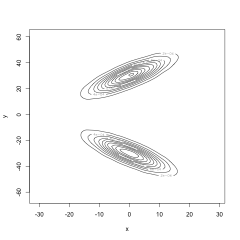
Suppose we have a mixture of two multivariate Gaussians. That is, we have two blobs, one pointed upward and the other pointed downward. A picture would probably help here:

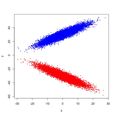
If we try to compute the correlation between $X$ and $Y$, we can see geometrically that we should get 0: recalling that for a two dimensional regression, the correlation and the slope of the line of best fit are related by a simple transformation, and noticing that the line of best fit would have a zero slope here², we get our result³.

But are $X$ and $Y$ independent? Clearly not: the more positive $X$ is, the more likely $Y$ is to be very large or very small, while the more negative $X$ is, the more likely $Y$ is to be near 0. That's a pretty clear dependence, and we can see it. But we don't have to stop at seeing: we can compute!

The quantity we want to compute is the mutual information between $X$ and $Y$, which I'll denote as $I[X; Y]$⁴. In particular, two random variables $X$ and $Y$ are independent if and only if (we get both directions now) their mutual information is zero. This seems mysterious (how do we get the other direction!) until we recall that the mutual information is the Kullback-Leibler divergence between their joint density and the product of their marginals,

\[ I[X; Y] = \iint\limits_{\mathcal{X}\times\mathcal{Y}} f_{X, Y}(x, y) \log_{2} \frac{f_{X, Y}(x, y)}{f_{X}(x)f_{Y}(y)} \, dA.\]

By inspection, we can see that if $f_{X, Y}(x,y)$ factors as $f_{X}(x) f_{Y}(y)$ (which gives us independence), we'll be computing logarithms of 1 throughout, which gives us zero overall for the integral. Thus, mutual information is really measuring how well the joint density factors, which is what we're interested in when it comes to independence.

After writing down the joint density for this data, we could compute the mutual information exactly and show that it's non-zero. Since I'm lazy, I'll let my computer do all of the work via an estimator for the mutual information. The tricky thing about computing information theoretic quantities is that the density itself is the object of interest, since we're computing expectations of it. Fortunately, we have ways of estimating densities⁵. That is, we can compute kernel density estimates $\hat{f}_{X}(x)$, $\hat{f}_{Y}(y)$, and $\hat{f}_{X, Y}(x, y)$⁶, and then plug them into the integral above to give us our 'plug-in' estimator for the mutual information.

Larry Wasserman, John Lafferty, and Han Liu even have a paper on how well we'll do using a method similar to this. I say 'similar' because I'm allowing the R software to automatically choose a bandwidth for the joint density and marginal densities, while they show that to achieve a parametric rate (in terms of the mean-squared error) of $n^{-1/2}$, we should take $h \asymp n^{-1/4}$ for both the univariate and bivariate density estimations⁷. A standard (apparently) result about bivariate density estimation via kernel density estimators is that we should take $h \asymp n^{-1/6}$ to obtain optimality. Thus, Wasserman et al.'s approach oversmooths compared to what we know should be done for optimal density estimation. But we have to keep in mind that our goal isn't to estimate the density; it's to estimate mutual information. A reminder that how we use our tools depends on the question we're trying to answer.

With 10000 samples to estimate the densities, we obtain the following estimator for the joint density:

Computing the marginals and multiplying them together, we see what the density would look like if $X$ and $Y$ really were independent:

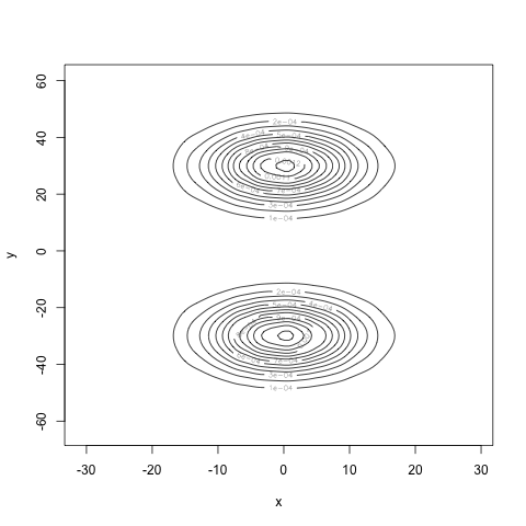
Very different! Finally, our estimate for the mutual information is 0.7, well away from 0. Our estimate for the correlation is 0.004, very close to zero. Our computations agree with our intuition: we have found a density for the pair $(X, Y)$ where $X$ and $Y$ are uncorrelated, but certainly not independent.

This exploration of correlation versus independence was originally motivated by a recent paper that made it all the way to a blurb in The Atlantic⁸. In it, the authors investigate whether properties of a researcher's Wikipedia entry are correlated with their prestige (using things like -index, number of years as a researcher, etc. as a proxy for prestige). They found no correlation. Which makes for a great story. But take a look at some of their evidence:

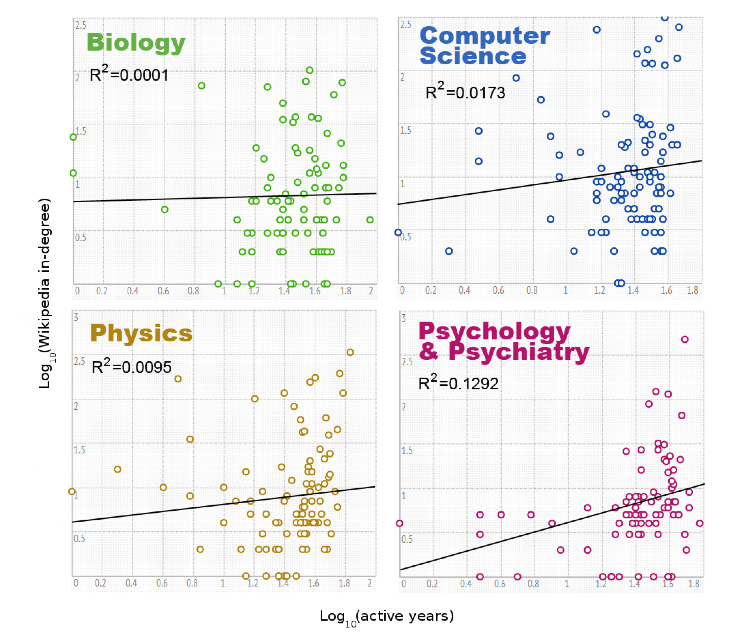
These are plots of the number of active years versus the in-degree of the Wikipedia articles for various authors on a log-log plot because, well, why not? They then fit a line of best fit because, well, that's what you do?⁹

Nevermind the log-log transformation (which destroys our intuitions about what a correlation would mean) and the fact that we have no reason to believe the expected behavior in the log-log space should be linear. (And never mind the atrocious $R^{2}$ values, and the fact that we shouldn't be using $R^{2}$ anyway!). Are the two things really uncorrelated? Its hard to say. But it's even harder to say they're independent, which is really what we'd like to know from the perspective of this study.

I don't expect to hear anyone citing "non-correlation is not independence" anytime soon. But it's something to keep in mind.

Given this fact, a better pneumonic might be "association is not causation."↩
Why? Through the magic of symmetric matrices and eigendecompositions, I've chosen the covariance matrices of each Gaussian to make the blobs exactly cancel each other out.↩
We could also compute out the correlation. But I only have so many integrals left in my life.↩
I sat in on an information theory course taught in our electrical engineering department where the professor used the notation $I[X \wedge Y]$. I do like that notation, since somehow it seems to more directly indicate the symmetric nature of mutual information. But I digress.↩
Though so so many scientists apparently don't know this. I've recently seen a lot of papers where people needlessly used histogram estimators for their densities. And they had a lot of data points. Why? I can only assume ignorance. Which makes me wonder what basic tools I am ignorant of. I spend every day trying to find out.↩
I'll leave it as an exercise why we estimate the marginals separately from the joint, rather than just estimate the joint and then marginalize.↩
Results like these are one of the many, many reasons why I love statistics. (And wish I was better at its theoretical aspects.) Not only do they show that an estimator exists that can achieve a very nice rate, but they also provide the correct bandwidth in order to achieve this rate. (Good) machine learning people provide insights like this too. Everyone else (i.e. 'scientists') attempt a method, see that it sort of works in a few examples, and then call it a day. I very much fall into that class. But I aspire for the precision of the statisticians and machine learners. In their defense, the scientists are probably busier worrying about their science to learn basic non-parametric statistics. But still...↩
Published in EPJ Data Science, whose tag line reads: "The 21st century is currently witnessing the establishment of data-driven science as a complementary approach to the traditional hypothesis-driven method. This (r)evolution accompanying the paradigm shift from reductionism to complex systems sciences has already largely transformed the natural sciences and is about to bring the same changes to the techno-socio-economic sciences, viewed broadly." How many buzz words can they fit in a single mission statement?↩
So this is data science!↩

MySQL for Statisticians

Over the past year, I've had to learn a bit of MySQL, an open source relational database management system, for my research. Our Twitter data is kept in MySQL databases for easy storage and access, and sometimes I have to get my hands 'dirty' in order to get the data exported into a CSV I can more readily handle.

Not having much formal training in computer science or software engineering, thinking about how to store data efficiently is new to me. I'm more used to thinking about data in the abstract, and hoping that, given enough time[^CS], any analysis I'd like to perform will run in (graduate school) finite time.

I started by learning MySQL in dribs and drabs, but recently I decided I should learn a new computational tool in the same way I learn everything else: from a book. While browsing through MySQL Crash Course, I had the realization that it would be nice if a book along the lines of MySQL for Statisticians existed[^google].

Why? The units of a MySQL database are very much like the units of a data matrix from classical statistics. Each MySQL database has 'tables,' where the columns of the tables correspond to different features / covariates / attributes, and the rows correspond to different examples.

Say you have a table with health information about all people in a given town. Each row would correspond to a person, and each column might correspond to their weight, height, blood pressure, etc. We can think of this as a matrix $\mathbf{X}$ of covariates, in which case we'd access all examples of a particular attribute by selecting the columns $\mathbf{x}_{j}$. Or we could think of this as a database, in which case (in the syntax of MySQL), we'd access the column by using

SELECT weight FROM pop_stats;

Knowing that an isomorphism (of sorts) exists between these two ways of looking at data makes a statisticians life a lot easier. This is probably a trivial realization, but it's one I wish I could have found more easily.

[^CS]: Caring about the computational complexity of a problem is something that computer scientists are much better at than general scientists. I've heard non-computer scientists claim that, "If it runs too slow, we'll just use C," as a rational way to handle any computing problem. But even the fastest C can't beat NP problems.

[^google]: A Google search did not reveal any current contenders.

The Trouble with Popularizing Science

I've developed a reputation as someone who gets annoyed at popularizations of science. From Nate Silver's book on statistics to many variations on quantum mechanics. They are all starting to get under my skin.

Why? I assume it's because I have started developed some expertise in a few branches of the physical and mathematical sciences. For example, popular books on biology don't typically bother me. I don't know nearly enough details to get annoyed by the generalizations and simplifications the authors indulge in.

An example of a popular science topic that annoys me to no end: the 'particle-wave' duality of light. Is light a particle? Or is it a wave? The popular science version says that light is both a particle and a wave. I would posit (and I'm not a physicist) that light is neither a particle nor a wave. It has both wave-like and particle-like properties. But a car has both cart-like and horse-like properties, and yet is neither of those two things. Why should light be forced to fit into a set of concepts developed in the 1700s?

Light is governed by a probability amplitude. Sure, understanding probability amplitudes requires a modicum of mathematical sophistication: one has to understand what a probability distribution is, what a complex number is, and the like. But these ideas are not so complicated. They can be grasped by anyone with a college-level mastery of calculus. In fact, when I took an intermediate-level quantum mechanics class in undergrad, I was shocked at how straightforward most of the math was: a little calculus, a little linear algebra, and a little probability theory. (And none of the hard parts from these topics.)

Popularizers of science have to walk a thin line between making science understandable and accurately representing its findings to the general public.

The End of Bayes?

I'll start with an excerpt by Cosma Shalizi:

This raises the possibility that Bayesian inference will become computationally infeasible again in the near future, not because our computers have regressed but because the size and complexity of interesting data sets will have rendered Monte Carlo infeasible. Bayesian data analysis would then have been a transient historical episode, belonging to the period when a desktop machine could hold a typical data set in memory and thrash through it a million times in a weekend.

— Cosma Shalizi, from here

Actually, you should leave here and read his entire post. Because, as is typical of Cosma, he offers a lot of insight into the history and practice of statistics.

For those in the know about Bayesian statistics¹, the ultimate object of study is the posterior distribution of the parameter of interest, conditioned on the data. That is, we go into some experiment with our own prejudices about what value the parameter should take (by way of a prior distribution on the parameter), do the experiment and collect some data (which gives us our likelihood), and then update our prejudice about the parameter by combining the prior and likelihood intelligently (which gives us our posterior distribution). This is not magic. It is a basic application of basic facts from probability theory. The (almost implicit) change of perspective that makes this sort of analysis Bayesian, rather than frequentist, is that we're treating the parameter as a (non-trivial) random variable: we pretend it's random, as a way to encode our subjective belief about the value it takes on. In math (to scare away the weak spirited),

\[ f(\theta | \mathbf{X}) = \frac{f(\mathbf{X} | \theta) f(\theta)}{\int f(\mathbf{X} | \theta') f(\theta') \, d \theta'}.\]

As Cosma points out in his post, the hard part of Bayesian statistics is deriving the posterior. Since this is also the thing we're most interested in, that is problematic. The strange thing about dealing in Bayesian statistics is that we rarely ever know the posterior exactly. Instead, we use (frequentist) methods to generate a large enough sample from something close enough to the actual posterior distribution that we can pretend we have the posterior distribution at our disposal. (Isn't Bayesian statistics weird²?) This is why Bayesians talk a lot about MCMC (Markov Chain Monte Carlo), Gibbs Sampling, and the like: they need a way to get at the posterior distribution, and pencil + paper will not cut it.

It's one thing to read about how these methods can fail in theory, but another to see it in practice. In particular, in the Research Interaction Team I attend on penalized regression, we recently read this paper on a Bayesian version of the LASSO³. In the paper, the authors never apply their method to the case where $p$ (the number of dimensions) is much greater than $n$ (the number of samples). Which is odd, since the frequentist LASSO really shines in the $p \gg n$ regime.

But then I thought about the implementation of the Bayesian LASSO, and the authors' 'neglect' became clear. To get a decent idea of the posterior distribution of the parameters of the Bayesian LASSO, the authors suggested sampling 100,000 times from the posterior distribution. But for each sample, they have to solve, in essence, a $p$ dimensional linear regression problem. For $p$ very large, this is a costly thing to do, even with the best of software. And they have to do this ten thousand times. Compare this to using coordinate descent for solving the frequentist LASSO, which is very fast, even for large $p$. And we only have to do this once.

In other words, we've hit up against the wall that Cosma alluded to in his post. The Bayesian LASSO is a clever idea, and its creators show in their paper that it outperforms the frequentist LASSO in the $p \approx n$ case⁴. But this case is becoming less and less the norm as we move to higher and higher dimensional problems. And MCMC isn't going to cut it.

If you're playing along at home, Bayesian statistics is this, and not this or this.↩
To be fair, in frequentist statistics, we pretend that our data are generated from an infinite population, and that our claims hold only over infinite repetitions of some experiment. I suppose it's all about what sort of weird you feel most comfortable with.↩
Somehow, this wasn't the first link to appear when I typed 'LASSO' into Google. Sometimes I have to remind myself that the real world exists.↩
Though they show performance based on simulations over ensembles of examples where $\boldsymbol{\beta}$ is fixed and randomness is introduced via the experiment. That is, they show its effectiveness in the frequentist case. Again, statistics is a weird discipline...↩

Mining Silver

tl;dr: Nate Silver really is a frequentist.

Yesterday, I had the chance to attend a lecture given by Nate Silver on his book The Signal and the Noise. I've written about Silver plenty of times in the past, but this was my first opportunity to see him speak in person.

Nate gave a very good talk. He was refreshingly modest. When he described his 538 work, he called his analysis 'just averaging the polls' (as I've said all along!).

But he was introduced as a 'leading statistician' (I'm sure he doesn't write his own PR blurb, but still...). He didn't talk much about the divide between Frequentist and Bayesian stats, but did put up Bayes's Rule and called it 'complicated math that you'll see in more and more stats journals, if you read such things.'

During the Q&A, I asked him about his attack on Frequentist statistics in his book¹, and where he got his viewpoint on statistics. He answered something like, "Mostly from a few papers I've read. Honestly, I don't talk to a lot of statisticians." Then he went on to say that he's 'philosophically a Bayesian' even though most of the methods he uses are Frequentist (like taking polling results and averaging them!). His words, not mine!

He went on a little longer, defending his view. But the main point I took away was that, to Nate, baby stats² and Frequentist statistics are synonymous, while the Bayesian philosophy is synonymous with anything that works.

This is a fine view to take, and it clearly works for Nate. It has the disadvantage that it's wrong³, but again, it works for Nate.

To recap: Nate is a very smart guy, and he's made a name for himself doing honest work. I just wish that as a "leading statistician" he would get his facts straight about the (very real) debate going on between Bayesian and frequentist statistics.

A taste: "Recently, however, some well-respected statisticians have begun to argue that frequentist statistics should no longer be taught to undergraduates. And some professions have considered banning Fisher's hypothesis test from their journals. In fact, if you read what's been written in the past ten years, it's hard to find anything that doesn't advocate a Bayesian approach." (p. 260 of The Signal and the Noise)

As a gut check, I looked at all of the articles published in Annals of Applied Statistics, Biostatistics, and Biometrika (three of the top statistics journals) in 2012, and computed the proportion of Bayesian articles. Only 42 out of 213 report on Bayesian methods, about 20%.↩
On the level of what is taught in AP Statistics.↩
Modern frequentist statistics is at least as sophisticated as Bayesian statistics, and many people have made arguments for frequentist methods over Bayesian methods.↩

All I Really Need for Data Analysis I Didn't Learned in Kindergarten — Non-Standard Stats and Statistical Schadenfreude

One of the fun things about reading scientific articles is seeing all of the ways that non-statisticians handle statistical questions¹. I'll try not to be too quick to cast aspersions on the scientists: they're busy focusing on their science, and haven't taken much time to bone up on any statistics past the most introductory stuff².

The real schadenfreude comes from a statistical analysis that seems reasonable on first blush, but that gives a wonky answer. The most recent example comes from a paper exploring statistical patterns in the communication behavior of individuals on Twitter. This work interested me due to its obvious connections to some work I've done.

The authors of this paper ask an interesting question: can we identify a statistical law that governs the time between tweets for users on Twitter? And if we can, can that law be used to distinguish between the accounts of regular users, corporations, and bots? Despite seeing power laws where there probably are none³, the authors do find that the statistical properties of the interarrival times of tweets have predictive power.

The strangeness occurs when the authors go about estimating the distribution of interarrival (or 'intertweet,' if we're feeling cheeky) times. The data, while continuous in reality comes binned (to the nearest second), already distorting the distribution we'd like to learn. The authors further distort (a kinder phrasing would be 'process') the data by further binning the raw data into log epochs. They then use a histogram estimator for the density, but use cubic spline interpolation to get values of the density between the discretized points.

Let's see what this looks like with a single realization of 100 normal⁴ random variates:

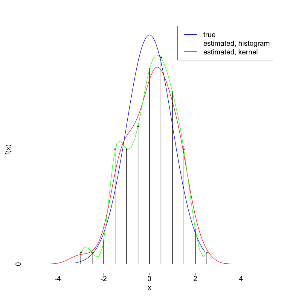
As we can see, the 'splined histogram' tends to give a more variable (too 'wiggly') density estimator than the standard kernel density estimation method. I think (though will not prove) that the splined histogram approach is consistent⁵, at least as long as we take the bin width to zero in a way depending on the sample size.

But the point is that we did a lot of extra work that only bought us a worse method. Kernel density estimation achieves the minimax risk up to a multiplicative constant, so we can't do much better with any non-parametric density estimation method. And there's no evidence this method should outperform the kernel density estimator's constant⁶.

One of the hallmarks of good science is asking interesting questions. The authors of this paper certainly do that. They could just use a bit more education in basic statistical inference⁷.

Similar in vein to finding clinicians who 'discover' the trapezoid rule.↩
Despite the existence of wonderful books that cover (almost) all of statistics.↩
Doing a similar analysis on my Twitter data, I found that the authors have probably made baby Gauss cry. In short, if you look at the tail of a log normal distribution, you can find something that looks very much like a power law, even when there is none.↩
As noted in the footnote above, the data are actually closer to log normal. But we can get back and forth between these two by exponentiating / logging, so I'll stick to the normal distribution since it's easier to visualize.↩
In the statistical sense. That is, in the limit of infinite data, it converges in probability to the true density of the data generating process.↩
I just realized that we could perhaps do cleverer things with this method. For example, instead of fixing the discretization, we could learn it adaptively using log-likelihood cross-validation. (The authors don't do this.) But this adds unnecessary bells and whistles to a junky car.↩
One of the reasons I sometimes bristle at the new phrase 'data science.' Data science seems to me, as an outsider, like statistics / computer science without the rigor. It need not be this. But that seems to be the direction it's currently heading.↩

Differences of Culture

I attended a few talks last week that highlighted the differences in culture that can exist between different academic disciplines.

In a talk on Monday, a group of students presented to a visiting professor. After listening to the students present, the professor always asked the students to summarize their work in the style they would use to explain their research to someone at a cocktail party. This is a good thing to point out to graduate students: we tend to get overly excited about our own research, and can miss the forest for the trees.

But that was the only question the professor would ask. Repeatedly. To all of the students. He didn't seem to pay much attention to the details of the presentations. He only wanted the big picture.

At a presentation in mathematics / statistics / computer science, there is a certain amount of work expected from the audience. The speaker will explain things, but the audience is expected to 'play along' and attempt to fill in some gaps as the presentation progresses. In my mind, there are two reasons for this. First, there isn't enough time to explain everything and cover enough material to get to the interesting parts. Second, the mental effort spent contemplating what the speaker is presenting keeps the audience engaged. It's the difference between reading a novel (entertaining, but requires little work) and a textbook.

I've noticed this when attending presentations outside of the mathematical sciences. The speaker focuses a lot on the big picture, but does not delve into the details of their methodology. They focus more on their results than how they got their results. Which leaves me uncomfortable: I am supposed to trust the speaker, but I have read too many crap scientific articles to immediately assume everyone has done their methodological due diligence.

I witnessed a different sort of cultural divide later in the week. I attended a seminar with an audience populated by mathematicians, physicists, and meteorologists. The presenter, a mathematician, freely used common mathematical notation like span (of a collection of vectors) and $C^{2}$ (the space of all twice continuously differentiable functions). The physicists and meteorologists had to ask for clarifications on these topics, not because they did not know them, but because they did not speak of them in such concise and precise terms. In the latter case, for instance, they probably had concepts of a function needing to be 'smooth,' where smooth is defined in some intuitive sense.

This reminds me of an excerpt from a review of textbooks that Richard Feynman undertook later his career. He volunteered to help the public school system of California decide on mathematics textbooks for their curriculum:

It will perhaps surprise most people who have studied these textbooks to discover that the symbol >> or << representing union and intersection of sets and the special use of the brackets and so forth, all the elaborate notation of sets that is given in these books, almost never appear in any writings in theoretical physics, in engineering, in business arithmetic, computer design, or other places where mathematics is being used. I see no need or reason for this all to be explained or taught in school. It is not a useful way to express one's self. It is not a cogent and simple way. It is claimed to be precise, but precise for what purpose?

— from New Textbooks for the 'New' Mathematics by Richard Feynman, excerpted from Perfectly Reasonable Deviations from the Beaten Track

Feynman wrote these words in the middle of the New Math turn in the education of mathematics in public schools. New Math focused on teaching set theory, a building block of much of modern mathematics, starting in elementary school. This wave of mathematics education did not last long in the US. It was certainly gone by the time I traversed the public school system. I didn't learn, formally, about sets until my freshman year course in Discrete Mathematics.

I think most mathematicians would find Feynman's statement that sets are "not a useful way to express one's self" very strange. At least for myself (and I'm the farthest thing from a pure mathematician), I find set theoretic notation extremely useful. But this might be a cultural thing. From the talk attended last week, the span is itself a set (the set of all linear combinations of some collection of vectors), as is $C^{2}$. And clearly the physicists and meteorologists have gotten along just fine without thinking of these things as sets, or using explicit set notation. Again, probably because they have some fuzzy, intuitive idea in their head for what these things mean.

Practical Inequalities — Hoeffding's Inequality

A friend had the following problem. His algorithm took as its input a random matrix, performed some operation on that matrix, and got out a result that either did or did not have some property. As the name implies, the random matrix is chosen 'at random.' In particular, each element is a independent and identically distributed normal random variable. There's a whole theory of random matrices, and things can get quite complicated.

Fortunately, for the problem at hand, we didn't need any of that complicated theory. In particular, what we're interested is the outcome of a certain procedure, and the inputs to that procedure are independent and identically distributed. Thus, the outputs are as well. Since the outcome either happens or does not, we really have that the outcomes are Bernoulli random variables, with some success probability $p$.

The question my friend had can be stated as: how many samples do I have to collect to say with some confidence that I have a good guess at the value of the success probability $p$? Anyone who has ever taken an intro statistics course knows that we can answer this question by invoking the central limit theorem. But that means we have to worry about asymptotics.

Let's use a nicer result. In particular, Hoeffding's inequality gives us just the tool we need to answer this question. Hoeffding's inequality¹ applies in a very general case. For Bernoulli random variables, the inequality tells us that if we compute the sample mean $\hat{p} = \frac{1}{n} \sum\limits_{i = 1}^{n} X_{i}$, then the probability that it will deviate by an amount $\epsilon$ from the true success probability $p$ is

\[ P\left(\left|\hat{p} - p\right| > \epsilon\right) \leq 2 \ \text{exp}(-2 n \epsilon^{2}).\]

Notice how this probability doesn't depend on $p$ at all. That's really very nice. Also notice that it decays exponentially with $n$ and the square of $\epsilon$: we don't have to collect too much data before we expect our approximation to $p$ to be a good one.

What we're interested in is getting the right answer, so flipping things around,

\[ P\left(\left|\hat{p} - p\right| \leq \epsilon\right) \geq 1 - 2 \ \text{exp}(-2 n \epsilon^{2}).\]

If we want to fix a lower bound of the probability of deviating from the true value $p$ by an amount $\epsilon$, call this value $\alpha$, then we can solve for $n$ and find

\[ n > - \frac{1}{2} \log\left(\frac{1 - \alpha}{2} \right)\epsilon^{-2}.\]

This gives us the number of times we'd have to run the procedure to be $100\alpha$% confident our result is within $\epsilon$ of the true value².

Of course, what we've basically constructed here is a confidence interval. But most people don't want to be bothered with 'boring'³ results from statistics like confidence intervals.

Inequalities make up the bread and butter of modern analysis. And with statistics being a branch of probability theory being a branch of measure theory, they also make for great tools in statistical analysis.↩
This reminded me that Hoeffding's inequality shows up in Probability Approximately Correct results in Statistical Learning Theory. Powerful stuff.↩
Though as we've seen, these results are far from boring, and involve some fun mathematics.↩

Kernel Density Estimation for Random Variables with Bounded Support — The Transformation Trick

Something that has bothered me since I started using kernel density estimators in place of histograms¹ is that I didn't see a natural way to deal with random variables with finite support. For example, if you're looking at the distribution of accuracy rates for some procedure, you know, a priori, that you can't get negative accuracy rates, or accuracy rates greater than 1 (if only!). Thus, the support of this random variable lies on $[0, 1]$, and any guess at the density function should also have support on $[0, 1]$.

The kernels used with kernel density estimators generally have support on the entire real line, so there's no way to use them 'out of the box' without getting non-meaningful values for parts of your estimator. If all you care about is the general shape of the density, that might not be a problem. But if you're really interested in capturing the exact shape, it is a problem.

To take the simplest example, suppose your data are generated from the uniform distribution on $[0, 1]$. In that case, we know the density function only has support on $[0, 1]$. But our naive kernel density estimator doesn't:

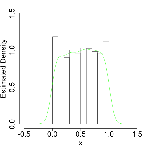
It more or less gets the shape right. But since it doesn't know it shouldn't bleed over the 'edges' at $x = 0$ and $x = 1$, it will always have a bias as these edges.

There are, I now know, numerous ways to get around this. My current favorite, which I learned about from here² after reading about the idea here, makes clever use of transformations of random variables.

Suppose we have a random variable with finite support. Call this random variable $X$. We know that using the vanilla kernel density estimator will not work for this random variable. But if we could deal with a transformed random variable $Y = g(X)$ that does take its support on the entire real line, and if the transformation $g$ is invertible, we can recover an estimator for the density of $X$ by first transforming our data with $g$, getting a kernel estimator for $Y = g(X)$, and then inverting the transformation.

To see how, recall that if $X$ has density $f_{X}$ and $Y$ has density $f_{Y}$ and $Y = g(X)$ with $g$ strictly monotonic so that we can invert it, then their densities are related by

\[ f_{Y}(y) = \frac{f_{X}(x)}{|g'(x)|}\bigg|_{x = g^{-1}(y)}\]

going one way and

\[f_{X}(x) = \left.\frac{f_{Y}(y)}{\left|\frac{d}{dy} \, g^{-1}(y)\right|} \right|_{y = g(x)}\]

going the other way.

But we have a way to get a guess at $f_{Y}(y)$: we can just use a kernel density estimator since we've chosen $g$ to give $Y$ support on the entire real line. If we replace $f_{Y}(y)$ with this estimator, we get an estimator for $f_{X}(x)$,

\[\hat{f}_{X}(x) = \left.\frac{\hat{f}_{Y}(y)}{\left|\frac{d}{dy} \, g^{-1}(y)\right|} \right|_{y = g(x)}.\]

And that's that.

To be a bit more concrete, suppose again that $X$ is uniform on $[0, 1]$. Then we need a transformation that maps us from $[0, 1]$ to $\mathbb{R}$³. A convenient one to use is the $\text{logit}$ function,

\[ \text{logit}(x) = \log \frac{x}{1-x}.\]

Inspection of this function shows that it takes $(0, 1)$ to $\mathbb{R}$, and is invertible with inverse

\[\text{logit}^{-1}(x) = \text{logistic}(x) = \frac{e^{x}}{1 + e^{x}}.\]

Computing a derivative and plugging in, we see that

\[ \hat{f}_{X}(x) = \frac{\hat{f}_{Y}(\text{logit}(x))}{x(1-x)}. \]

Since $\hat{f}_{Y}(y)$ is the sum of a bunch of kernel functions, it's like we placed a different kernel function at each point $x$. This gives us a much better estimate at the density:

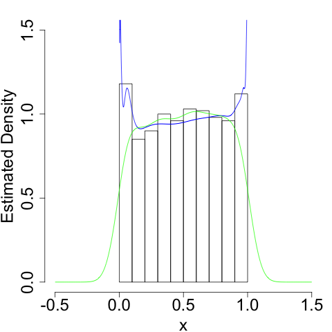
We still run into problems at the boundaries (infinities are hard), but we do a much better job of getting the shape (the flatness) of the density correct.

We can of course pull this trick for random variables with support on, say, $[0, \infty)$. In this case, we use $g(x) = \log(x)$, and we get

\[ \hat{f}_{X}(x) = \frac{\hat{f}_{Y}(\text{log}(x))}{x}. \]

For example, we can use this if $X$ is exponentially distributed:

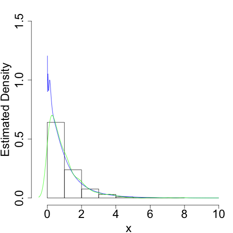
Again, we do a much better job of capturing the true shape of the density, especially near its 'edge' at $x = 0$.

And you generally should.↩
As with most of the cool things about statistics I know, I learned this from Cosma Shalizi. Hopefully he won't mind that I'm answering his homework problem on the inter webs.↩
Technically, we'll use a transformation that maps us from $(0, 1)$ (the open interval) to $\mathbb{R}$. In theory, since $X = 0$ and $X = 1$ occur with measure zero, this isn't a problem. In practice, we'll have to be careful how we deal with any $1.0$ and $0.0$s that show up in our data set.↩