Kernel Density Estimation for Random Variables with Bounded Support — The Transformation Trick
Something that has bothered me since I started using kernel density estimators in place of histograms1 is that I didn't see a natural way to deal with random variables with finite support. For example, if you're looking at the distribution of accuracy rates for some procedure, you know, a priori, that you can't get negative accuracy rates, or accuracy rates greater than 1 (if only!). Thus, the support of this random variable lies on \([0, 1]\), and any guess at the density function should also have support on \([0, 1]\).
The kernels used with kernel density estimators generally have support on the entire real line, so there's no way to use them 'out of the box' without getting non-meaningful values for parts of your estimator. If all you care about is the general shape of the density, that might not be a problem. But if you're really interested in capturing the exact shape, it is a problem.
To take the simplest example, suppose your data are generated from the uniform distribution on \([0, 1]\). In that case, we know the density function only has support on \([0, 1]\). But our naive kernel density estimator doesn't:
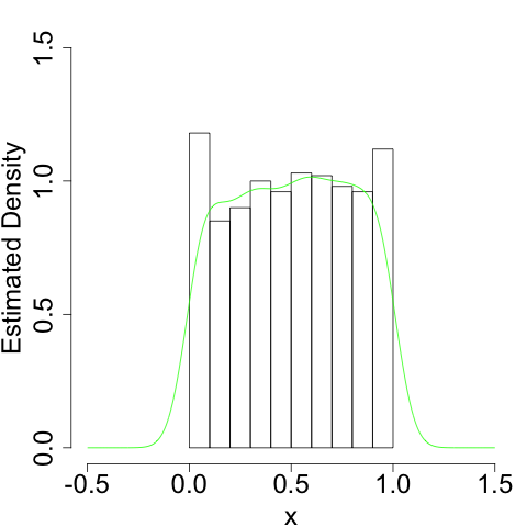
It more or less gets the shape right. But since it doesn't know it shouldn't bleed over the 'edges' at \(x = 0\) and \(x = 1\), it will always have a bias as these edges.
There are, I now know, numerous ways to get around this. My current favorite, which I learned about from here2 after reading about the idea here, makes clever use of transformations of random variables.
Suppose we have a random variable with finite support. Call this random variable \(X\). We know that using the vanilla kernel density estimator will not work for this random variable. But if we could deal with a transformed random variable \(Y = g(X)\) that does take its support on the entire real line, and if the transformation \(g\) is invertible, we can recover an estimator for the density of \(X\) by first transforming our data with \(g\), getting a kernel estimator for \(Y = g(X)\), and then inverting the transformation.
To see how, recall that if \(X\) has density \(f_{X}\) and \(Y\) has density \(f_{Y}\) and \(Y = g(X)\) with \(g\) strictly monotonic so that we can invert it, then their densities are related by
\[ f_{Y}(y) = \frac{f_{X}(x)}{|g'(x)|}\bigg|_{x = g^{-1}(y)}\]
going one way and
\[f_{X}(x) = \left.\frac{f_{Y}(y)}{\left|\frac{d}{dy} \, g^{-1}(y)\right|} \right|_{y = g(x)}\]
going the other way.
But we have a way to get a guess at \(f_{Y}(y)\): we can just use a kernel density estimator since we've chosen \(g\) to give \(Y\) support on the entire real line. If we replace \(f_{Y}(y)\) with this estimator, we get an estimator for \(f_{X}(x)\),
\[\hat{f}_{X}(x) = \left.\frac{\hat{f}_{Y}(y)}{\left|\frac{d}{dy} \, g^{-1}(y)\right|} \right|_{y = g(x)}.\]
And that's that.
To be a bit more concrete, suppose again that \(X\) is uniform on \([0, 1]\). Then we need a transformation that maps us from \([0, 1]\) to \(\mathbb{R}\)3. A convenient one to use is the \(\text{logit}\) function,
\[ \text{logit}(x) = \log \frac{x}{1-x}.\]
Inspection of this function shows that it takes \((0, 1)\) to \(\mathbb{R}\), and is invertible with inverse
\[\text{logit}^{-1}(x) = \text{logistic}(x) = \frac{e^{x}}{1 + e^{x}}.\]
Computing a derivative and plugging in, we see that
\[ \hat{f}_{X}(x) = \frac{\hat{f}_{Y}(\text{logit}(x))}{x(1-x)}. \]
Since \(\hat{f}_{Y}(y)\) is the sum of a bunch of kernel functions, it's like we placed a different kernel function at each point \(x\). This gives us a much better estimate at the density:
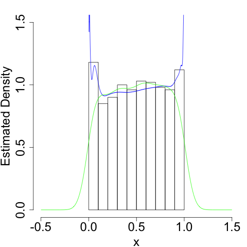
We still run into problems at the boundaries (infinities are hard), but we do a much better job of getting the shape (the flatness) of the density correct.
We can of course pull this trick for random variables with support on, say, \([0, \infty)\). In this case, we use \(g(x) = \log(x)\), and we get
\[ \hat{f}_{X}(x) = \frac{\hat{f}_{Y}(\text{log}(x))}{x}. \]
For example, we can use this if \(X\) is exponentially distributed:
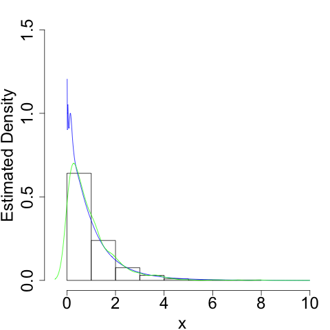
Again, we do a much better job of capturing the true shape of the density, especially near its 'edge' at \(x = 0\).
And you generally should.↩
As with most of the cool things about statistics I know, I learned this from Cosma Shalizi. Hopefully he won't mind that I'm answering his homework problem on the inter webs.↩
Technically, we'll use a transformation that maps us from \((0, 1)\) (the open interval) to \(\mathbb{R}\). In theory, since \(X = 0\) and \(X = 1\) occur with measure zero, this isn't a problem. In practice, we'll have to be careful how we deal with any \(1.0\) and \(0.0\)s that show up in our data set.↩