So You Think You Can Statistics: Overlapping Confidence Intervals, Statistical Significance, and Intuition
Attention Conservation Notice: I begin a new series on the use of common sense in statistical reasoning, and where it can go wrong. If you care enough to read this, you probably already know it. And if you don’t already know it, you probably don’t care to read this. Also, I’m cribbing fairly heavily from the Wikipedia article on the t-test, so I’ve almost certainly introduced some errors into the formulas, and you might as well go there first. Also also: others have already published a paper and written a Masters thesis about this.
Suppose you have two independent samples, \(X_{1}, \ldots, X_{n}\) and \(Y_{1}, \ldots, Y_{m}\). For example, these might be the outcomes in a control group (\(X\)) and a treatment group (\(Y\)), or a placebo group and a treatment group, etc. An obvious summary statistic for either sample, especially if you’re interested in mean differences, is the sample mean of each group, \(\bar{X}_{n}\) and \(\bar{Y}_{m}\). It is then natural to compare the two and ask: can we infer a difference in the averages of the populations from the difference in the sample averages?
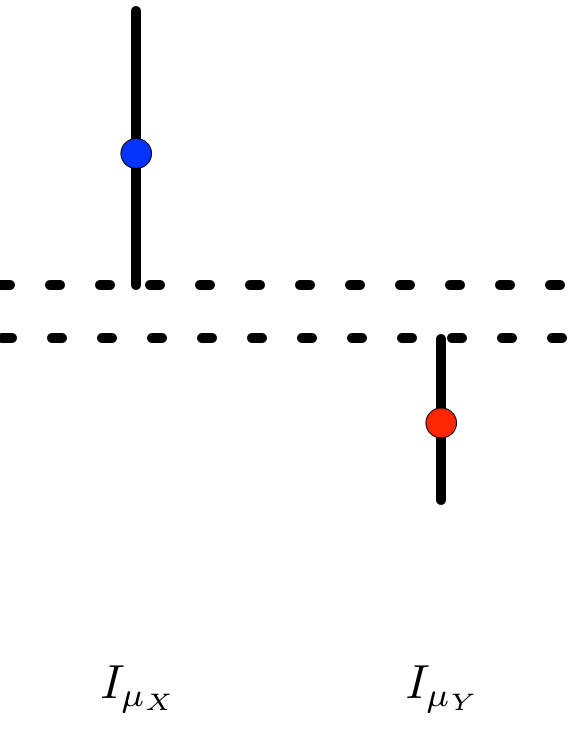
If a researcher is clever enough to use confidence intervals rather than P-values, they may begin by constructing confidence intervals for \(\mu_{X}\) and \(\mu_{Y}\), the (hypothetical) population means of the two samples. For reasonably sized samples that are reasonably unimodal and symmetric, a reasonable confidence interval is based on the \(T\)-statistic. Everyone learns in their first statistics course that the \(1 - \alpha\) confidence intervals for the population means under the model assumptions of the \(T\)-statistic are
\[I_{\mu_{X}} = \left[\bar{X}_{n} - t_{n - 1, \alpha/2} \frac{s_{X}}{\sqrt{n}}, \bar{X}_{n} + t_{n-1, \alpha/2} \frac{s_{X}}{\sqrt{n}}\right]\]
and
\[I_{\mu_{Y}} = \left[\bar{Y} _{m}- t_{m - 1, \alpha/2} \frac{s_{Y}}{\sqrt{m}}, \bar{Y}_{m} + t_{m - 1, \alpha/2} \frac{s_{Y}}{\sqrt{m}}\right],\]
respectively, where \(s_{X}\) and \(s_{Y}\) are the sample standard deviations. These are the usual ‘sample mean plus or minus a multiple of the standard error’ confidence intervals. It then seems natural to see if these two intervals overlap to determine whether the population means are different. This sort of heuristic, for example, is described here and here. Yet despite the naturalness of the procedure, it also happens to be incorrect[1].
To see this, consider the confidence interval for the difference in the means, which in analogy to the two confidence intervals above I will denote \(I_{\mu_{X} - \mu_{Y}}\). If we construct the confidence interval by inverting[2] Welch’s t-test, then our \(1 - \alpha\) confidence interval will be
\[I_{\mu_{X} - \mu_{Y}} = \left[ (\bar{X}_{n} - \bar{Y}_{m}) - t_{\nu, \alpha/2} \sqrt{\frac{s_{X}^{2}}{n} + \frac{s_{Y}^{2}}{m}}, \\ (\bar{X}_{n} - \bar{Y}_{m}) + t_{\nu, \alpha/2} \sqrt{\frac{s_{X}^{2}}{n} + \frac{s_{Y}^{2}}{m}} \right]\]
where the degrees of freedom \(\nu\) of the \(T\)-distribution is approximated by
\[\nu \approx \frac{\left(\frac{s_{X}^{2}}{n} + \frac{s_{Y}^{2}}{m}\right)^{2}}{\frac{s_{X}^{4}}{n^{2}(n - 1)} + \frac{s_{Y}^{4}}{m^{2} (m - 1)}}.\]
This is a[3] reasonable confidence interval, where it would be a very good confidence interval if you’re willing to assume that the two populations are exactly normal but have unknown and possibly different standard deviations. This is again a ‘sample mean plus or minus a multiple of a standard error’-style confidence interval. How does it relate to the ‘overlapping confidence intervals’ heuristic?
Well, if we’re only interested in using our confidence intervals to perform a hypothesis test for whether we can reject (using a test of size \(\alpha\)) that the population means are not equal, then our heuristic says that the event \(I_{\mu_{X}} \cap I_{\mu_{Y}} = \varnothing\) (i.e. the individual confidence intervals do not overlap) should be equivalent to \(0 \not \in I_{\mu_{X} - \mu_{Y}}\) (i.e. the confidence interval for the difference does not contain \(0\)).
Well, when does \(I_{\mu_{X}} \cap I_{\mu_{Y}} = \varnothing\)? Without loss of generality, assume that \(\bar{X}_{n} > \bar{Y}_{m}\). In that case, the confidence intervals do not overlap precisely when the lower endpoint of \(I_{\mu_{X}}\) is greater than the upper endpoint of \(I_{\mu_{Y}}\),
That is,
\[\bar{X}_{n} - t_{n-1, \alpha/2} \frac{s_{X}}{\sqrt{n}} > \bar{Y}_{m} + t_{m - 1, \alpha/2} \frac{s_{Y}}{\sqrt{m}},\]
and rearranging,
\[\bar{X}_{n} - \bar{Y}_{m} > t_{n-1, \alpha/2} \frac{s_{X}}{\sqrt{n}} + t_{m - 1, \alpha/2} \frac{s_{Y}}{\sqrt{m}}. \hspace{1 cm} \mathbf{(*)}\]
And when isn’t 0 in \(I_{\mu_{X} - \mu_{Y}}\)? Precisely when the lower endpoint of \(I_{\mu_{X} - \mu_{Y}}\) is greater than 0, so
\[\bar{X}_{n} - \bar{Y}_{m} - t_{\nu, \alpha/2} \sqrt{\frac{s_{X}^{2}}{n} + \frac{s_{Y}^{2}}{m}} > 0\]
Again, rearranging
\[\bar{X}_{n} - \bar{Y}_{m} > t_{\nu, \alpha/2} \sqrt{\frac{s_{X}^{2}}{n} + \frac{s_{Y}^{2}}{m}}. \hspace{1 cm} \mathbf{(**)}\]
So for the heuristic to ‘work,’ we would want \(\mathbf{(*)}\) to imply \(\mathbf{(**)}\). We can see a few reasons why this implication need not hold: the \(t\)-quantiles do not match and therefore cannot be factored out, and even if they did, \(\frac{s_{X}}{\sqrt{n}} + \frac{s_{Y}}{\sqrt{m}} \neq \sqrt{\frac{s_{X}^{2}}{n} + \frac{s_{Y}^{2}}{m}}\). We do have that \(\frac{s_{X}}{\sqrt{n}} + \frac{s_{Y}}{\sqrt{m}} \geq \sqrt{\frac{s_{X}^{2}}{n} + \frac{s_{Y}^{2}}{m}}\) by the triangle inequality. So if we could assume that all of the \(t\)-quantiles were equivalent, we could use the heuristic. But we can’t. Things get even more complicated if we use a confidence interval for the difference in the population means based on Student’s \(t\)-test rather than Welch’s.
As far as I can tell, the triangle inequality argument is the best justification for the non-overlapping confidence intervals heuristic. For example, that is the argument made here and here. But this is based on confidence intervals from a ‘\(Z\)-test,’ where the quantiles come from a standard normal distribution. Such confidence intervals can be justified asymptotically, since we know that a sample mean standardized by a sample standard deviation will converge (in distribution) to a standard normal by a combination of the Central Limit Theorem and Slutsky’s theorem[4]. Thus, this intuitive approach can give a nearly right answer for large sample sizes in terms of whether we can reject based on overlap. However, you can still have the case where the one sample confidence intervals do overlap and yet the two sample test says to reject. See more here.
My introduction to the overlapping confidence interval heuristic originally arose in the context of this journal article on contrasting network metrics (mean shortest path length and mean local clustering coefficient) between a control group and an Alzheimers group. The key figure is here, and shows a statistically significant separation between the two groups in the Mean Shortest Path Length (\(L_{p}\) in their notation, right most figure) at certain values of a thresholded connectivity network. Though, now looking back at the figure caption, I realize that their error bars are not confidence intervals, but rather standard errors[5]. So, we can think of these as 84% confidence intervals for a large enough sample. They will be about half as long as a 95% confidence interval. But even doubling them, we can see a few places where the confidence intervals do not overlap and yet the two sample \(t\)-test result is not significant.
Left as an exercise for the reader: A coworker asked me, “If the individual confidence intervals don’t tell you whether the difference is (statistically) significant or not, then why do we make all these plots with the two standard errors?” For example, these sorts of plots. Develop an answer that (a) isn’t insulting to non-statisticians and (b) maintains hope for the future of the use of statistics by non-statisticians.
-
By ‘incorrect,’ here I mean that we can find situations where the heuristic will give non-significance when the analogous two sample test will give significance, and vice versa. To quote Cosma Shalizi, writing in a different context, “The conclusions people reach with such methods may be right and may be wrong, but you basically can’t tell which from their reports, because their methods are unreliable.” ↩
-
I plan to write a post on this soon, since a quick Google search doesn’t turn up any simple explanations of the procedure for inverting a hypothesis test to get a confidence interval (or vice versa). Until then, see Berger and Casella’s Statistical Inference for more. ↩
-
A because you can come up with any confidence interval you want for a parameter. But it should have certain nice properties like attaining the nominal confidence level while also being as short as possible. For example, you could take the entire real line as your confidence interval and capture the parameter value 100% of the time. But that’s a mighty long confidence interval. ↩
-
We don’t get the convergence ‘for free’ from the Central Limit Theorem alone because we are standardizing with the sample, rather than the population, standard deviation. ↩
-
There is a scene in the second PhD Comics movie where an audience member asks a presenter, “Are your error bars standard deviations or standard errors?” The presenter doesn’t know the answer, and the audience is aghast. After working through this exercise, this joke is both more and less funny. ↩