A Heuristic for Thinking About Iterated Expectations

I'm reading this paper on sparse additive models for a Research Interaction Team in penalized regression. I'll be giving a fifty-ish minute presentation on it to a group of statistics, computer science, and mathematics graduate students. So far, I'm having the enjoyable experience of having my understanding of the paper arrive in stages¹. For this to happen, I have to read the paper several times, over the course of several days. This is something I should do more of in general.

After giving the paper a first go, I realized that I should probably learn more about additive models before I read about sparse additive models. My go-to person for clear exposition on statistical methods is Cosma Shalizi, and fortunately he's writing a book on advanced data analysis (i.e. modern statistics) from an elementary point of view (i.e. mine). In particular, he has a very nice chapter on additive models. As usual, he motivates why the popular method for fitting them, called backfitting, makes sense in the first place, and then works through several nice examples of additive models 'in the wild.'

In his initial derivation of why we might use backfitting, he provides a very nice intuitive way to think about the law of total / iterated expectation². The law of total expectation, in its simplest form, says that

\[ E[Y] = E[E[Y | X]].\]

That is, computing the average value of $Y$ is equivalent to computing the average value that $Y$ takes given each value of $X$, and then averaging over $X$³. That seems reasonable. We can also extend the result to conditioning on more than one random variable. For example, in regression, we're frequently interested in $E[Y | X]$, the expected value of our outcome $Y$ given a particular value of a covariate / feature $X$. But suppose we have additional information, $Z$, that we could consider. How is $E[Y | X]$ related to $Z$? Iterated expectation tells us

\[ E[Y | X] = E[E[Y | X, Z] | X].\]

(Generally, the more things we condition on, the easier we make our lives, since once we've conditioned on a random variable we can treat it as a (conditional) constant and pull it outside of some of the expectations.)

This version is less clear, just by looking at it. But Cosma gives a nice verbal description of what's going on here. Basically, we can continue to condition on as many other random variables as we want, as long as we ultimately average over those newly conditioned random variables. We can see that happening above: we've conditioned on a new random variable $Z$, but at the end of the day we average over it by taking the outer $E[\cdot | X]$.

The original example can be framed in this way if we allow for an abuse of notation. In particular,

\[ E[Y | \{ \}] = E[E[Y | X] | \{\}]\]

where the empty set is there to remind us that we're not conditioning on anything.

As opposed to the unenjoyable experience on the first pass through the paper where I had no idea what was going on.↩
Iterated expectation, like many things in practical probability, involves conditioning. And like many things in probability theory, life becomes easier when the manipulations involving conditioned quantities become intuitive.↩
I first learned this result in my undergraduate probability theory course. I had no idea why the professor seemed so enamored with it. Now I do.↩

Parametric, Semiparametric, and Nonparametric Models

In reading the paper related to this post¹, I came across a new class of statistical models I hadn't heard of before: semiparametric models.

We're all familiar with parametric models, even if we don't call them that. We introduce students to these types of models in statistics courses: the normal model, the exponential model, the Poisson model, etc.² For example, we can specify a normal random variable by writing down its density function

\[ f_{X}(x) = \frac{1}{\sqrt{2 \pi \sigma^{2}}} \text{exp} \left[ \frac{1}{2 \sigma^{2}}(x - \mu)^{2} \right], x \in \mathbb{R}. \]

From this density function, we can compute all of the quantities we might like to about some random variable $X$ with this density. But notice that all we need to specify the density are the mean $\mu$ and variance $\sigma^{2}$ (or 'location' and 'scale,' in more general terminology). We can wrap those both up into a parameter vector $\theta = (\mu, \sigma^{2}),$ and we trivially see that this vector living in a subset of $\mathbb{R}^{2}$. It lives in a finite space.

But if we want to, say, talk about a model that incorporates all densities with mean 0, we can't specify such a model with a single parameter. We know the mean is 0, but that's it. And that doesn't fully specify our density. Instead, we can think of the density as living in an infinite dimensional vector space.

But first, let's take a more common example to make this clear. Think about quadratic polynomials,

\[ a x^{2} + b x + c, \text{ where } (a, b, c) \in \mathbb{R}^{3}.\]

This family of quadratic polynomials exhibit the properties of a vector space (closure under addition, existence of a zero element, etc.)³. This seems obvious once we wrap up the coefficients into the triple $(a, b, c)$; in fact, the space of quadratic polynomials is isomorphic to $\mathbb{R}^{3}.$

The important thing to notice here is that, to specify a quadratic function, we need only specify three real numbers, $(a, b, c)$. Thus, this vector space is finite-dimensional⁴.

As an opposing example, consider the space of continuous functions. We know we can approximate a continuous function using polynomials of finite degree, and can even exactly recover the continuous function using a Taylor expansion. But in that case, to specify the function, we need to list out the coefficients from the Taylor expansion, $(a_{0}, a_{1}, a_{2}, \ldots),$ and for an arbitrary continuous function, we might need infinitely many of these. (Consider, for example, $e^{x}$.) Thus, the space of continuous functions is an infinite-dimesional vector space.

In statistics, when we can't specify a model using a finite set of parameters, we call the resulting model non-parametric. This name is a little confusing. Non-parametric models often have parameters. For example, kernel density estimators have the smoothing parameter $h$. As we saw, a better name for these types of models might be 'infinite dimensional.' But that sounds scarier.

Modern statistics has a lot of non-parametric models to choose from⁵. Which is good, since as I mentioned in the first note below, we usually have no reason to think nature should follow a parametric model we can write down. For density estimation, we have kernel density estimators, which do as well as we could hope. For regression, we have splines, kernels, and much more.

Semiparametric models lie in the grey area between parametric and non-parametric models. To specify a semiparametric model, you must specify both a finite-dimensional vector of parameters, and an infinite-dimensional function. As a simple example, consider a regression model

\[ Y = \boldsymbol{\beta}^{T} \mathbf{X} + g(Z) + \epsilon.\]

The first bit, $\boldsymbol{\beta}^{T} \mathbf{X}$ should be familiar from linear regression: we have covariates / features $\mathbf{X}$ and a parameter vector $\boldsymbol{\beta}$. $\boldsymbol{\beta}$ is the finite-dimensional part of the model. The second bit, $g(Z)$, is an arbitrary function, and makes up the infinite-dimensional part of the model. Of course, we know neither $\boldsymbol{\beta}$ nor $g$, and must infer them from data.

Something I hope to write about in a bit, since it's related to some reading I've been doing about sampling with networks.↩
It's worth asking the question: why should nature follow a simple model that 18th and 19th (and 20th) century mathematicians, statisticians, and physicists could write down? Sometimes, we have good reasons, both theoretical and physical, to assume a certain model. Often, we don't.↩
Most people learn about vector spaces for the first time in linear algebra. The thing that frequently catches them off guard is that things like the quadratic are non-linear polynomials. But our attention is now on the coefficients $(a_{n}, \ldots, a_{0})$, not the variable $x$. The polynomials are linear in the coefficients.↩
It's technically finite because it has a finite set of basis vectors.↩
From my very limited vantage point, the two main contributions of modern statistics have been non-parametric methods and methods for dealing with high-dimensional inference.↩

Tweets, Metadata, and Other Controversial Topics — And a New Paper

First, a pretty picture.

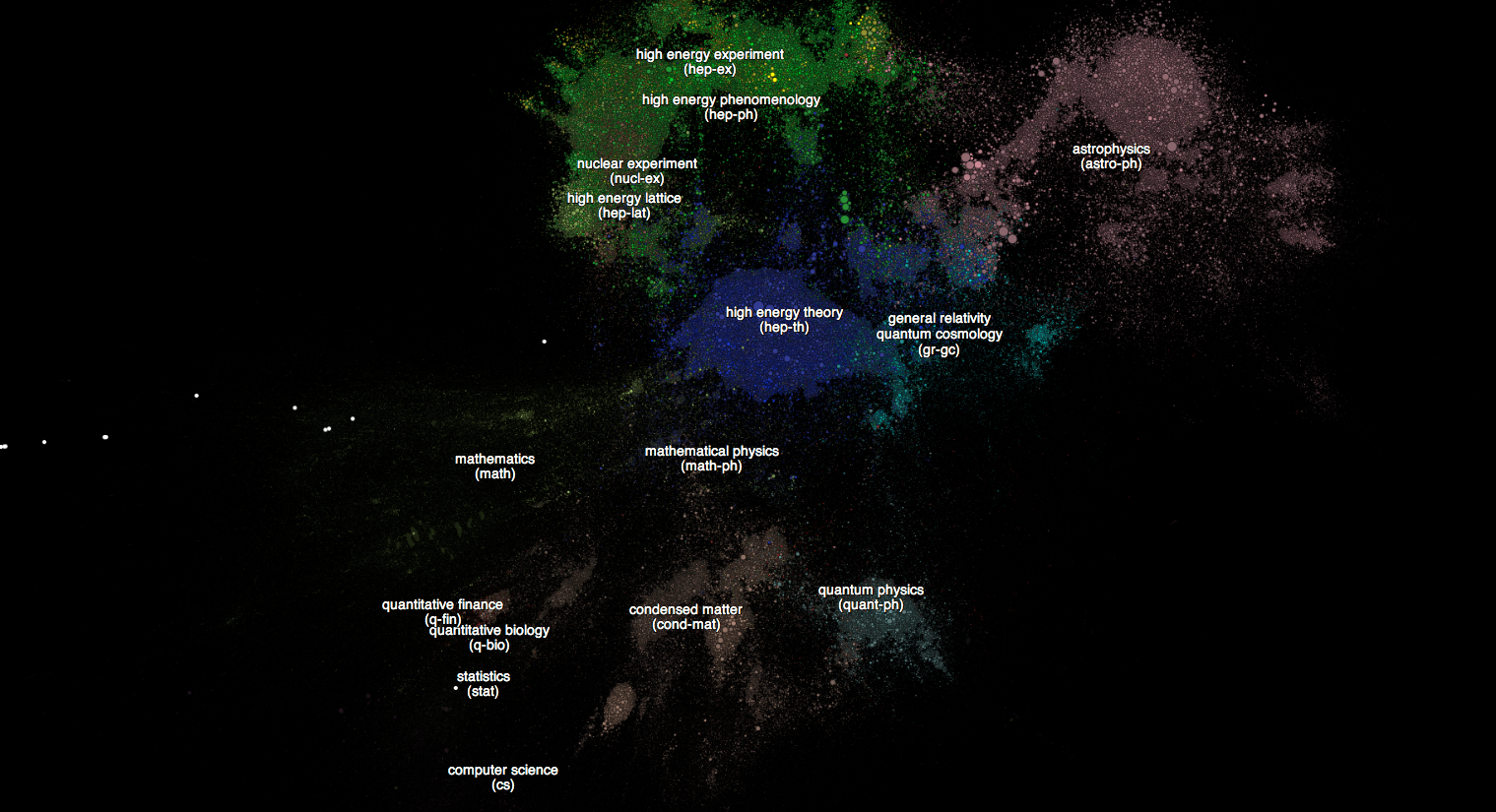
These clouds of points represent 866,543 papers from the arXiv, an open access scientific publishing site first created in 1991¹. This map of the arXiv universe is maintained by Damien George and Rob Knegjens over at paperscape. It's hot off the presses, having only been released this month. I found out about it from Sean Carroll's blog.

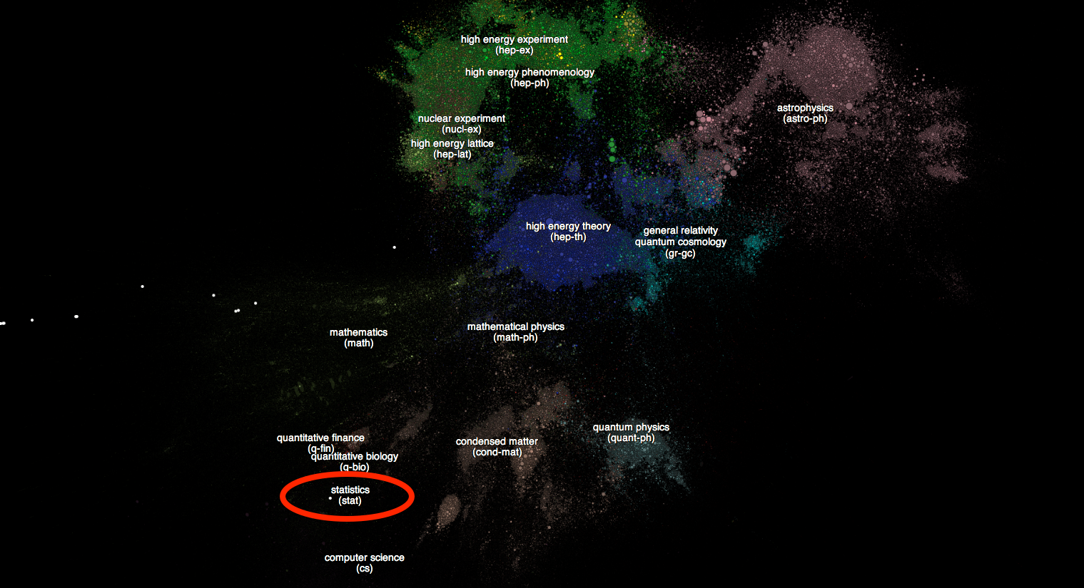
The natural first thing to do when you come across such a map is to search for oneself². I only have a single paper housed on the arXiv, from work I did this winter on prediction in social media. That paper shows up as a lonely blip in the statistics cluster of the arXiv:

I'm happy³ to have it situated there. I'm an aspiring statistician, of the weakest sort: in the tool using, not the tool making, sense.

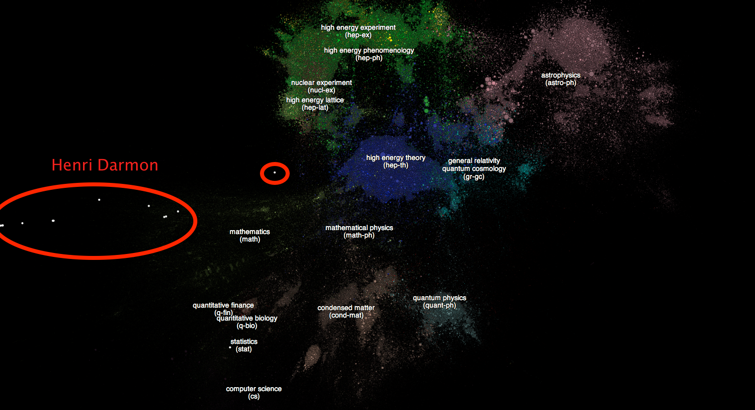
You'll notice another sprinkling of white points, in the offshoot from the math cluster. I knew those papers didn't correspond to any work I did, despite my academic home in the University of Maryland's Mathematics department. Upon closer investigation with paperscape, I determined these papers were written by or contained references to a Canadian mathematician by the name of Henri Darmon⁴:

Henri is a number theorist at McGill University, and according to this page, "[o]ne of the world's leading number theorists, working on Hilbert's 12th problem." One of his inventions is Darmon points, something useful enough to have symposiums about.

Since my interests don't frequently stray into number theory, I don't imagine either of us has to worry about name pollution. (Especially Henri.) I'll have to start working on my own version of Darmon *.

Clearly, physics dominates the arXiv 'galaxy.' The arXiv started as a repository for high energy physics papers. I didn't realize how comparatively few papers from other disciplines get published to the arXiv.↩
Actually, the zeroth thing I did was search for my advisor.↩
During an exit interview after an internship at Oak Ridge that lead to this paper, I told the head PI that I would never use probabilistic models again. Further evidence that we shouldn't trust our past selves to have half a clue about what our future selves will want.↩
Darmon is a relatively common French name. At least, that was the impression during a trip to Paris where a new acquaintances attempt to find me on Facebook was hindered by the prevalence of David Darmon's in France. My entire life I thought I had a rare name, but the rareness is very much geographically determined.↩

How to Compare Communities Using Variation of Information

Attention conservation notice: To compare communities in a network determined by differing methods, use Variation of Information, or some other statistic derived from the confusion matrix. But really, variation of information has a lot of nice properties.

Sometimes I write posts for this blog to answer questions I posed to Google without (immediate) answers¹. I found myself asking such a question in mid-August.

The question: how can you compare the communities in a network determined by two (or more) different approaches?

Because I can't help myself, the basic setup is this. You have a graph $G = (V, E)$ where $V$ is the set containing the vertices of the graph and $E$ is a binary operator determining whether two vertices are connected. That is, for two vertices $u, v \in V$, we have $uEv = 1$ if $u$ and $v$ are connected, and $uEv = 0$ if they are not. These connections are often encoded in an adjacency matrix $\mathbf{A}$ where the $(i, j)$ element of $\mathbf{A}$ is $a_{ij} = (\mathbf{A})_{ij} = v_{i}Ev_{j}$. (We'll assume an undirected network for now.) That is, $\mathbf{A}$ is a matrix with binary entries that encodes the pairwise connections.

Once you have a collection of vertices $V = \{ v_{1}, \ldots, v_{|V|}\}$, you might want to partition these nodes somehow. Usually we partition them based on the structural properties of the network, which are wrapped up in either $E$ or $\mathbf{A}$. For example, we might take a modularity-based approach² and try to group together nodes so that there are more connections falling between the nodes in a particular community than from those nodes out to other communities. This approach was pioneered by Mark Newman and my advisor. We usually call the sets of nodes making up this partition communities (if we're working in some sort of social science) or modules (otherwise). The name 'community' should make sense: if we consider a social network, we expect people within a community (say, a club or organization) to have more connections to the members inside that community than without. For a prosaic example, consider the fact that at the University of Maryland, most of my friends are in the Mathematics department. (Fortunately, many of my friends in the Mathematics department don't suffer from this affliction.)

I won't focus on how to go about finding these communities. There are lots of methods out there. Which raises the question: if we use two different community detection algorithms, what is a useful way to compare how similar the communities are between the partitions each algorithm supplies? That is, we want some way to tell if we're getting basically the same communities with the two algorithms, and if so, how similar.

A person might go through and compare community by community, partition by partition, to see if the communities 'look' similar. This approach would work, but it doesn't scale well and its hard to automate. But the intuition is right. Instead of looking at individual nodes within the communities, we'll look at how much the different communities overlap in terms of all of their nodes.

Again, to be a bit more formal, suppose we have two partitions $\mathcal{C} = \{C_{1}, \ldots, C_{|\mathcal{C}|}\}$ and $\mathcal{C}' = \{C'_{1}, \ldots, C'_{|\mathcal{C}|}\}$ where each $C_{i}$ is a collection of nodes. We can compute the confusion matrix $\mathbf{N}$ from these two partitions, where \[ (\mathbf{N})_{kk'} = |\mathcal{C} \cap \mathcal{C}'|.\] In short, for a community $k$ from partition $\mathcal{C}$ and a community $k'$ from partition $\mathcal{C}'$, we count up the number of overlapping members (the number of nodes that appear in both partitions). The confusion matrix most naturally shows up in classification problems, where we have true and predicted class labels for each item in our data set, and we want to see how 'confused' our prediction algorithm got, overall. For the question we're interested in, we don't necessarily have 'true' communities (unless we do), but the confusion matrix still serves its purpose: it tells us how much overlap there is between the communities in each partition.

Once we have $\mathbf{N}$, which will be a $|\mathcal{C}| \times |\mathcal{C}'|$ matrix, we recognize that we have something very close to joint probability mass function that tells us the probability that a node, chosen at random from our network, lies in community $k$ and community $k'$. To get there, we just need to divide all of the entries in $\mathbf{N}$ by $|V|$, the number of nodes in our network. This does give us an (empirical) probability mass function \[p(k, k') = \frac{1}{|V|}(\mathbf{N})_{k k'}.\]

What sort of question do we want to ask using this distribution? Remember our motivating question: how different are the partitions induced by the two community detection algorithms? If they're very different, knowing what community a node is in from partition $|\mathcal{C}|$ shouldn't tell you what community the node is in $|\mathcal{C}|$. On the other hand, if the induced partitions are very similar, then the opposite is the case: knowing the community from one partition might completely fix the community from the other partition. (Say, if the two partitions are identical.) We're talking about knowledge and 'surprise,' so it shouldn't be too shocking that the way we'll formalize this intuition is via (what else?) information theory.

Jumping to the punchline, the quantity we're interested in is called the variation of information between two random variables $X$ and $Y$, and we'll denote it by $VI[X; Y]$. For our problem, $X \in \{ 1, 2, \ldots, |\mathcal{C}|\}$ is the community from $\mathcal{C}$ for a node chosen at random from the network, and $Y \in \{ 1, 2, \ldots, |\mathcal{C}'|\}$ is the community from $\mathcal{C}'$ for a node chosen at random. Thus, we see that $p(k, k')$ is exactly the joint distribution for $(X, Y)$, that is \[ P(X = k, Y = k') = p(k, k'),\] since we've assumed that each node is chosen with equal probability.

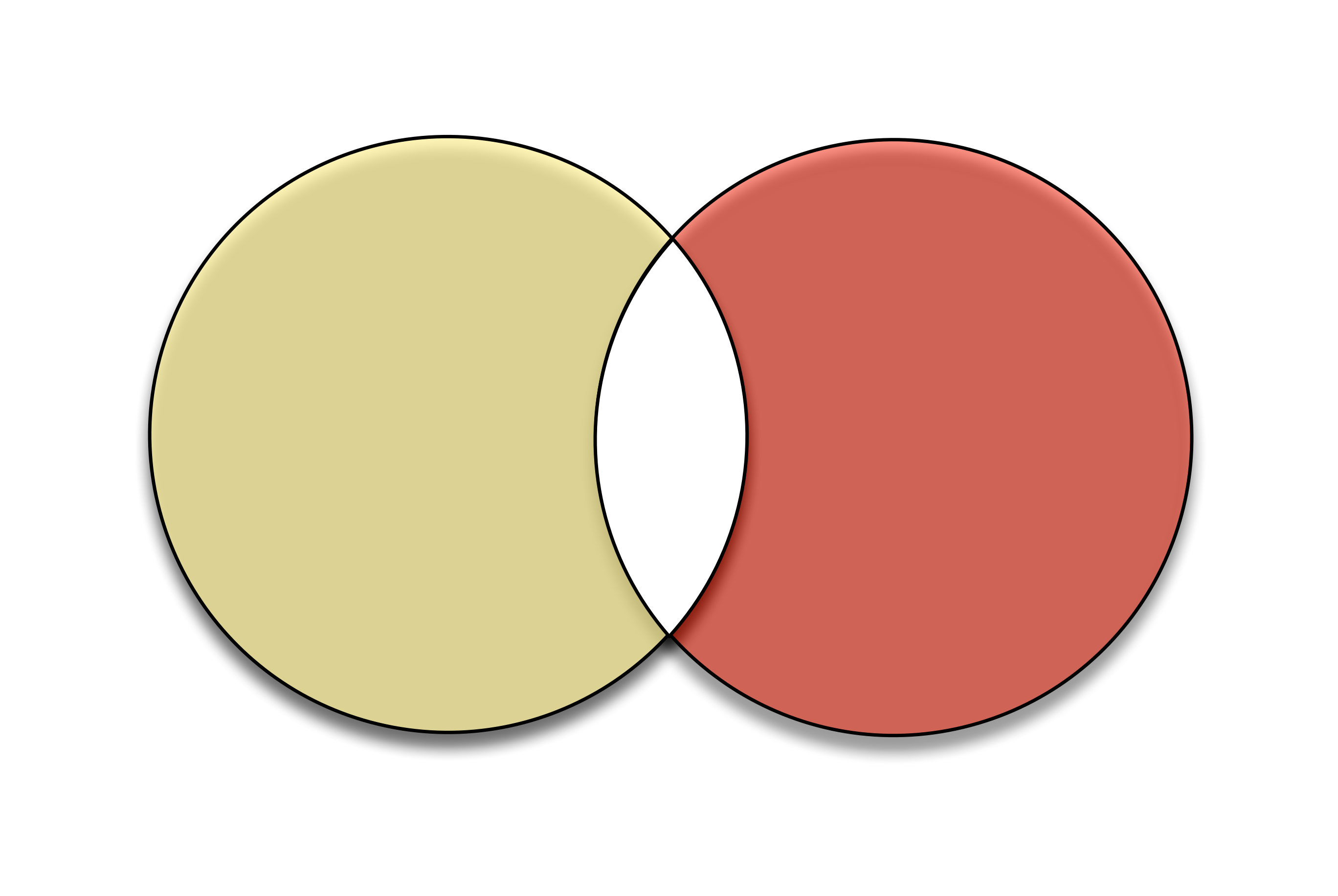
We saw how to represent the relationship between information theoretic quantities using information diagrams, a particular application of Venn diagrams. Variation of information makes up a simple portion of the information diagram: it's the non-overlapping portions of the Venn diagram,

From this, we can see that there are various equivalent definitions of variation of information, in particular \[\begin{align} VI[X; Y] &= H[X | Y] + H[Y | X] \\ &= H[X] + H[Y] - 2 I[X; Y] \\ &= H[X, Y] - I[X; Y]. \end{align}\]

Thinking about this, we see that variation of information will be maximal when $X$ tells us nothing about $Y$ and $Y$ tells us nothing about $X$ (the two circles are disjoint, so their mutual information is zero), which is precisely when the two partitions are as different as possible. Similarly, the variation of information is zero when the two circles completely overlap.

We saw that, almost by construction, variation of information matches the intuitive definition we might come up with for defining similarity between two partitions. But it also satisfies a bunch of nice mathematical properties. For example, it's a metric on the space of possible partitions, in the formal sense: it's non-negative, symmetric, and satisfies the triangle inequality. This means that it really does match our intuition of distance (since the concept of a metric is just a formalization of this intuition). Moreover, we can bound it above by $2 \log_{2}{|V|}$, so we can normalize it between 0 and 1, everyone's favorite continuum.

Two examples: how do you compute the density of a random variable after application of a non-monotonic transformation? How is the survival function used to compute expectations? These now show up (when logged in under my Google account) on the top page. And given the traffic to my website, a lot of people find the second result (the 'Darth Vader rule') useful. I owe the internet this. I used to end up at this site every time I wanted to write a piecewise function in LaTeX.↩
Though this isn't always called for. See this paper by Aaron Clauset on the pitfalls and perils of using modularity maximization in real-world contexts. This paper should be required reading for anyone interested in community detection!↩

Of Camping and Information Lost

Suppose you have a lock with three slots on it, and each slot can take one of the digits 0 through 9. After opening the lock, you'll want to thwart any evil doers by somehow randomizing the digits. (Otherwise, why have the lock?) The best strategy is to scramble each of the digits. But suppose we take a lazier strategy and choose one of the digits at random and scramble it. How much information has our hypothetical safe cracker lost about the actual lock combination by this randomization process?

This problem (after some mathematization) falls squarely in the realm of information theory. We can rephrase it as follows: if we have a lock combination $X$ drawn uniformly from $\{ 0, 1, \ldots, 9\}^{3}$, and then we generate $Y$ by the scrambling process above, how much information have we lost about $X$ once we know $Y$? Recalling that the mutual information, the amount of information we gain about $X$ by knowing $Y$ (or vice versa) is

\[ I[X; Y] = H[X] - H[X | Y], \]

we see that the quantity we're interested in computing is really $H[X | Y]$, the information we've 'lost.'

Let's start by simplifying things a bit to sure up our intuition. Suppose that instead of a decimal-based lock, we have a binary lock with three bits. We'll take the initial lock combination to be uniform on $\{0, 1\}^{3}$. Now suppose we use a simple procedure to randomize our lock. Instead of choosing one of the bits at random, we'll always randomize the first bit. Intuition tells us that the randomization process should lead to the loss of one bit of information about the true combination $X$. How can we check that our intuition is guiding us correctly?

To compute $H[X | Y]$, we need the conditional mass function $p(x | y)$, the probability the original lock combination was $x$ given that we observed the scrambled combination $y$. What we know going into the problem are $p(x)$, since we've assumed the original lock was chosen completely randomly¹, and $p(y | x)$, since we know that the scrambled combination will take the values $0x_{1}x_{2}$ and $1x_{1}x_{2}$ with equal probability, where $x_{0}x_{1}x_{2}$ is the original lock combination. We get $p(x|y)$ from these in the usual way, by noting that \[ \begin{align} p(x | y) &= \frac{p(y | x) p(x) }{p(y)} \\ &= \frac{\frac{1}{2} \cdot \frac{1}{8}}{\frac{1}{8}} = \frac{1}{2} \end{align}\] for all $(x, y)$ that 'make sense' (i.e. those where $x$ could be the unscrambled version of $y$), and zero otherwise. We already saw that $p(x | y)$ will be $\frac{1}{2}$ for such $(x, y)$, and since $x$ is uniform on $\{0, 1\}^{3}$, each of the 8 possible combinations has equal probability, namely $\frac{1}{8}$. Moreover, since $X$ is uniform, given our scrambling procedure it follows that $Y$ will also be uniform.

We have everything we need (again, $p(x | y)$) to compute $H[X | Y]$. We can visualize $p(x | y)$ as a stochastic matrix $\mathbf{W}$, with each row corresponding to a particular value of $y$ and each column corresponding to a particular value of $x$ and each entry corresponding to $p(x | y)$. For each $y$ value, there are two possible $x$ values, and there are 8 possible $y$ values. Thus, $\mathbf{W}$ will have 16 non-empty entries, each with probability equal to $\frac{1}{2}$. Thus, we can easily compute \[\begin{align} H[X | Y] &= -\sum_{(x, y) \in \{0, 1\}^{3} \times \{ 0, 1\}^{3}} p(x,y) \log_{2} p(x | y) \\ &= -16\cdot\frac{1}{16} \cdot \log_{2} \frac{1}{2} \\ &= 1, \end{align}\] which gives us 1 bit, as we expected.

Now to the case of interest: where we randomize which bit we scramble. Intuitively, we imagine that this should lead to more information lost than in the case where we always scramble the same bit. Thus, the information lost should certainly be greater than 1 bit.

And now I've lost steam. The procedure for finding $H[X | Y]$ in this case is exactly the same. We can already specify $p(x)$ and $p(y | x)$, though $p(y | x)$ will be a bit more complicated. In particular, $Y$ will no longer be uniform on $\{ 0, 1\}^{3}$, so we'll have to compute $p(y)$ by marginalizing down from $p(x, y) = p(x) p(y | x)$. We also have to be a little bit more careful about the number of non-zero entries in our new $\mathbf{W}$. But once we do what amounts to bookkeeping, we'll find that for this randomization procedure, \[ H[X | Y] = 1.7925\ldots \text{ bits},\] which is an improvement over 1 bit, but not as good as 3 bits (which we would get if we completely randomized the lock each time). We have bought ourselves 0.7925 more bits of security by randomizing which bit we scramble.

Knowing people, the original combination probably wasn't chosen completely randomly. For instance, in the decimal lock case, I imagine people are more hesitant to use combinations with repeated digits like '111' or '222.'↩

Ones Place in the arXivs of History

First, a pretty picture.

I'm happy³ to have it situated there. I'm an aspiring statistician, of the weakest sort: in the tool using, not the tool making, sense.

Clearly, physics dominates the arXiv 'galaxy.' The arXiv started as a repository for high energy physics papers. I didn't realize how comparatively few papers from other disciplines get published to the arXiv.↩
Actually, the zeroth thing I did was search for my advisor.↩
During an exit interview after an internship at Oak Ridge that lead to this paper, I told the head PI that I would never use probabilistic models again. Further evidence that we shouldn't trust our past selves to have half a clue about what our future selves will want.↩
Darmon is a relatively common French name. At least, that was the impression during a trip to Paris where a new acquaintances attempt to find me on Facebook was hindered by the prevalence of David Darmon's in France. My entire life I thought I had a rare name, but the rareness is very much geographically determined.↩

All I Really Need for Data Analysis I Learned in Kindergarten — Venn, Shannon, and Independence

Venn¹ diagrams are one of the first graphical heuristics we learn about in elementary (middle? high?) school. They're a convenient way to represent sets², and allow for the easy visualization of set operations like intersection and union.

Once we have sets, we can consider a measure³ on top of those sets, and we have ourselves the beginnings of measure theory. And thanks to our good friend Andrey Kolmogorov, we can then employ them in probability theory, which is really nothing but measure theory restricted to a space with measure 1.

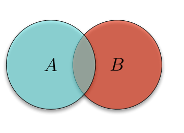
Elementary probability theory was my first formal introduction to the usefulness of Venn diagrams. If you have two events $A$ and $B$, and want to talk about probabilities associated with them, you can draw a general two-circle Venn diagram,

and use that diagram to get out any quantity involving intersections and unions⁴. For example, the probability that $A$ or $B$ occurs is the probability $P(A \cup B)$, which we see is just the 'area' of the union of the two sets. Similarly, the probability that $A$ and $B$ occur $P(A \cap B)$ is the area of the intersection of $A$ and $B$, which we can get by computing $P(A) + P(B) - P(A \cup B)$.

This is all old news, and common fair for any introductory probability course. But as I said in one of the footnotes, these sorts of Venn diagrams can't represent any sort of conditional probability, which we're often interested. A common pitfall of a beginning probabilist is to think that disjointness means independence⁵. Recall that two events $A$ and $B$, both with probability greater than 0, are independent if

\[ P(A \cap B) = P(A) P(B) \]

or equivalently if

\[ P(A | B) = P(A) \]

\[ P(B | A) = P(B). \]

In words, this means that two events are independent if the probability of one occurring doesn't depend on the other occurring. This seems like a reasonable enough definition. But what about when two events are disjoint? Are they independent?

If two events are disjoint, then $P(A \cap B) = 0$. But, with some manipulation, we see

\[ P(A | B) = \frac{P(A \cap B)}{P(B)} = 0 \neq P(A), \]

since we assumed that $P(A) > 0$. Thus, $A$ is not independent of $B$. In fact, they're as dependent as they could get: once we know that $A$ happens, we know for sure that $B$ did not happen.

I found this result so striking that, at one point during a intermediate probability theory course, I wrote in my notebook, "There is no way to show independence with Venn diagrams!" It seems like we should be able to, but remember that Venn diagrams only allow us to show things about intersections and unions, not conditioning.

But I was only part right about this conclusion. It turns out a slightly different sort of Venn diagram⁶ perfectly captures these conditional relationships. To get there, we need to expand our probabilistic language to include information theory⁷. For two random variables $X$ and $Y$⁸, we will specify their joint probability mass function by $p(x,y)$. Then their joint entropy can be computed as

\[ \begin{align} H[X, Y] &= - E[\log_{2} p(X, Y)] \\ &= -\sum_{(x, y) \in \mathcal{X} \times \mathcal{Y}} p(x, y) \log_{2} p(x,y) \end{align} \]

and their marginal entropies $H[X]$ and $H[Y]$ can be computed in the same way using the marginal probability mass functions $p(x)$ and $p(y)$. We'll also need two more objects (and a third guest star), namely the conditional entropies $H[X | Y]$ and $H[Y | X]$, where the first is defined as

\[ H[X | Y] = -E[\log_{2} p(X | Y)]\]

and the second is defined in the obvious way⁹.

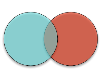
To get the Venn diagram, we start with an empty Venn diagram

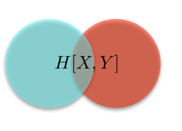
where the circle on the left contains the 'information' in $X$ and the circle on the right contains the 'information' in $Y$¹⁰. Thus, it makes sense that if we consider the union of these two circles, we should get the information contained in both $X$ and $Y$, namely the joint entropy $H[X, Y]$, and we do:

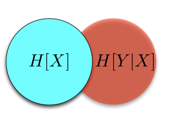
We've already called the circle on the left the information in $X$, so it makes sense that this should correspond to the entropy of $X$, $H[X]$. And it does. But what do we get if we take away information in $X$ from the information we have about both $X$ and $Y$? As expected, we get the information left in $Y$ after we've conditioned on $X$, namely $H[Y | X]$:

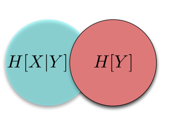
The same results hold if we fix our attention on $Y$:

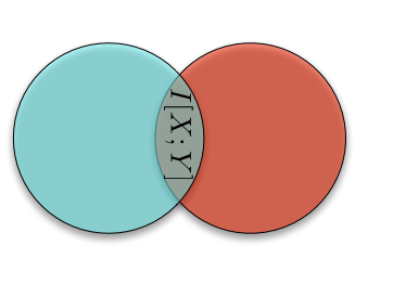
The only portion we haven't explicitly named is the portion in the middle: the intersection of the information in $X$ and the information in $Y$. This part of the information diagram is called, unsurprisingly, the mutual information between $X$ and $Y$, $I[X; Y]$:

Now we have a name for all of the basic players in elementary information theory, and a way to compute them from each other. For example, the mutual information is

\[ I[X; Y] = H[X] + H[Y] - H[X, Y]. \]

(In the same way that we got $P(A \cap B)$ above.)

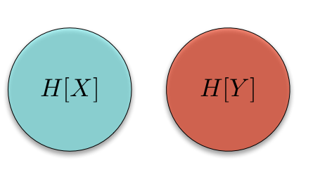
Now we're finally ready to show independence with our new Venn diagram. First, recall a fact: two random variables $X$ and $Y$ are independent if and only if their mutual information is zero. This means that two marginal informations in our information diagram have to have zero overlap:

The informations have to be disjoint! (Which is exactly what we mistakenly thought we were getting at with the probability Venn diagrams.)

These information diagrams are nothing new, and have found great success in explicating the properties of stochastic processes in general. Strangely, they only receive the briefest mention in most introductions to information theory¹¹. Hopefully with time, these simple objects from our primary school days will permeate information theory and beyond.

Poor John Venn, who did a lot of work in mathematics, logic, and statistics, mostly gets recalled for his invention of Venn diagrams. As an example of some of his other work: "[Venn] is often said to have invented one of the two basic theories about probability, namely the frequency account. The 'fundamental conception,' he wrote, is that of a series which 'combines individual irregularity with aggregate regularity'." — Ian Hacking, from page 126 of The Taming of Chance↩
At least for three or fewer sets.↩
Where, for the purposes of this post, we'll take 'measure' here literally: think of how you might measure the length, area, volume, etc. of an object. Things are really more complicated, but we'll sweep those complications under the rug for now.↩
But not those properties that involve conditioning. For that, we'll have to introduce a different Venn diagram, as we'll see in a bit.↩
This is yet another case of our everyday language failing to map to the formal language of mathematics.↩
Which, like all things in elementary information theory, may be found in Cover and Thomas's Elements of Information Theory. In this case, on page 22 of the second edition.↩
And start to talk about random variables instead of events. But what is a random variable but another way at looking at an induced probability space?↩
For simplicity, we'll only talk about discrete random variables, i.e. those that take on a countable set of values.↩
The nice thing about information theory is that everything is defined in the 'obvious' way: for whatever quantity you're interested in, compute the expectation of the associated mass function and you're done.↩
We've already seen why it makes sense to talk about 'information' and 'entropy' almost interchangeably, especially for discrete random variables.↩
In the introductory information theory course I sat in on, the professor didn't mention them at all. And as I said, to my knowledge Cover and Thomas only covers them on a single page.↩

Statistics, Data Science, and Silver

I've commented in the past on the choice of Nate Silver as the invited speaker at this year's Joint Statistical Meeting. I have been very critical of Silver, mostly because of some choice words he made about modern statistics in his popular science book The Signal and the Noise.

Silver's address to the JSM has come and gone, and I have to say, I'm very impressed with how he handled the opportunity. Since I didn't attend the JSM, and the JSM don't seem to broadcast its presentations (for shame!), I have gotten my coverage of Silver's talk second hand. Let's take this post as a pretty good indication of what Silver chose to talk about.

First, I'm happy that Silver admitted he is not a statistician. I've written in the past about the difference between a statistician and someone who uses statistics. We need both sorts of people, just as we need mechanical engineers and car mechanics, and computer scientists and software engineers.

The rest of his talk addressed the role of statistics in journalism, which is certainly a topic Nate Silver knows a great deal about. Again, see this post at Revolutions for the eleven points Silver covered. Almost all of them are admonishments for those journalists who would also become quantitatively literate. This is great news, especially given the current state of the journalistic enterprise.

Apparently during the Q&A (mediated via Twitter!), Silver was asked for his thoughts about the possible distinction between data science and statistics. To my surprise, he commented that data science is a "sexed up" term for statistician. Which I'm of two minds about, given the divide I've decided to impose between statisticians and people who use statistics. At various times in the past year, I've made the claim that data science is the same thing as statistics, but I would also hesitate to claim that all data scientists are statisticians. And many of the more notable data scientists seem to share that hesitation. That's a strange contradiction to deal with: a field is really a sub-discipline of statistics, and yet its main practitioners are not statisticians.

I suppose this isn't too perplexing. Large parts of empirical science could be considered sub-branches of statistics. For instance, 'econometrics' is a fancy name for applying statistical models to economic problems. Psychometrics is another case of the exact same situation, except considering psychological measurements. Data science has just abstracted a field to anything that involves data (though 'data' itself is perhaps ill-defined), and thus must necessarily use statistics. (Since statistics is the branch of mathematical engineering that deals with noisy data coming from the real world.) But that doesn't make those people statisticians.

I've said in the past that I aspire to be a statistician, and I still stand by that aspiration. But I also aspire to hone my schlep skills so that I can answer cool questions about the real world that no one has thought to ask. There's certainly room for both sorts of skills, and no reason why a person with one should necessarily have the other. As this article explains, a PhD prepares you for doing research, but not necessarily for doing industry-scale data science.

First Languages and Boltzmann Machines — Part Two: Statistics

We consider a random vector $\mathbf{X} = (X_{1}, \ldots, X_{N_{v}}) \in \{ 0, 1\}^{N_{v}}$. The use of $N_{v}$ for the number of random variables in our vector is suggestive. In fact, $\mathbf{X}$ is a Markov Random Field with $N_{v}$ vertices. We'll assume that the probability mass function for $\mathbf{X}$ is given by¹

\[ p(\mathbf{x}; \boldsymbol{\Theta}, \boldsymbol{\theta}_{0}) = \frac{1}{Z} \text{exp} \left \{ \sum_{j} \theta_{0j} x_{j} + \sum_{(j, k) \in \mathcal{E}} \theta_{jk} x_{j} x_{k} \right \}, \]

where $\mathcal{E}$ is an edge list, with $(j,k) \in \mathcal{E}$ only if there exists an edge between random variable $j$ and random variable $k$. (Remember that we implicitly have a Markov Random Field in the background, so we also have an undirected graphical model with nodes and (undirected) edges.)

Borrowing from our physicist friends, the joint mass function can be rewritten in a much more compact form using matrix/vector notation as

\[ p(\mathbf{x}; \boldsymbol{\Theta}, \boldsymbol{\theta}_{0}) = \frac{1}{Z} \text{exp} \left \{ \boldsymbol{\theta}^{T}_{0} \mathbf{x} + \frac{1}{2} \mathbf{x}^{T}\boldsymbol{\Theta} \mathbf{x} \right \} = \frac{1}{Z} \text{exp} \left \{ E(\mathbf{x}; \boldsymbol{\Theta}, \boldsymbol{\theta}_{0}) \right \}.\]

Again, the $E$ here should be suggestive. We can think of this as some sort of energy function of $\mathbf{x}$. We can do this, but we won't, for now. I'm writing down a particular statistical model. We'll see some of the consequences of that model later. I warned you that my first language is statistics.

You'll notice the $\frac{1}{Z}$ out front of our probability mass function. It's there to make sure that our sum over all $\mathbf{x} \in \{ 0, 1\}^{N_{v}}$ gives us 1, as it must. That is, it's a normalization constant. Physicists have a different name for it: they call it the partition function. It gets a fancier name in statistical mechanics because, when a distribution takes a form like $p(\mathbf{x}; \boldsymbol{\Theta}, \boldsymbol{\theta}_{0})$ above, you can derive certain properties of $p$ by manipulations with the partition functions (taking logs, derivatives, etc.). For completeness, the partition function is

\[ Z = \sum_{\mathbf{y} \in \{ 0, 1\}^{N_{v}}} \text{exp} \left \{ E(\mathbf{y}; \boldsymbol{\Theta}, \boldsymbol{\theta}_{0}) \right \}\]

where we introduce a dummy summation variable $\mathbf{y}$ here so as not to confuse ourselves with the $\mathbf{x}$ showing up as the argument to $p(\mathbf{x}; \boldsymbol{\Theta}, \boldsymbol{\theta}_{0})$.

And with that, we're done. We've fully specified this particular model, since we can compute anything we might possibly want to know about $\mathbf{X}$ using $p(\mathbf{x}; \boldsymbol{\Theta}, \boldsymbol{\theta}_{0})$. For instance, we might want to compute it's mean value, in which case for each $X_{j}$ in $\mathbf{X}$, we would compute²

\[ E[X_{j}] = \sum_{\mathbf{x} \in \{ 0, 1\}^{N_{v}}} p(\mathbf{x}; \boldsymbol{\Theta}, \boldsymbol{\theta}_{0}) x_{j}, \]

collect those together into a vector, and we would have $E[\mathbf{X}]$. The same goes for the covariance matrix, etc. We're not really done, since to compute any of these things, we'll have to sum over a (possibly) very large set $\{ 0, 1\}^{N_{v}}$. This set has cardinality $2^{N_{v}}$, which grows exponentially in $N_{v}$. That's bad news for computational tractability.

But fortunately, being statisticians, we can get around this by sampling³ from $p(\mathbf{x}; \boldsymbol{\Theta}, \boldsymbol{\theta}_{0})$. Or, as it's usually called in this context, using Monte Carlo methods. We can approximate any expectation by drawing a random sample $\mathbf{X}^{(1)}, \mathbf{X}^{(2)}, \ldots, \mathbf{X}^{(N)}$ from $p(\mathbf{x}; \boldsymbol{\Theta}, \boldsymbol{\theta}_{0})$ and computing

\[ E[g(\mathbf{X})] \approx \frac{1}{N} \sum_{i = 1}^{N} g(\mathbf{X}^{(i)}).\]

By the law of large numbers, our sample average will converge on the true average, and we're done.

Of course, how we sample from $p(\mathbf{x}; \boldsymbol{\Theta}, \boldsymbol{\theta}_{0})$ is an another question. A standard approach is to use Gibbs sampling. Gibbs sampling, in essence, generates a sample from a multivariate distribution by successively sampling from its conditional distributions. That is, it's easy to show⁴ that for a fixed $X_{j}$, the conditional distribution, conditioning on all other $X_{k}$ making up $\mathbf{X}$, is

\[ P(X_{j} = 1 \ | \ \mathbf{X}_{-j} = \mathbf{x}_{-j}) = \frac{1}{1 + \text{exp} \left\{ - \theta_{j} - \sum_{(j, k) \in \mathcal{E}} \theta_{k} x_{k}\right\} } \]

where $\mathbf{X}_{-j} = (X_{1}, \ldots, X_{j-1}, X_{j+1}, \ldots, X_{N_{v}})$ is the random vector once we've removed the random variable of interest $X_{j}$. Since, given $\mathbf{X}_{-j}$, this distribution is easy to sample from, we just iterate through all of the $j$, successively updating the value of $X_{j}$ based on this probability. The succession of $\mathbf{X}^{(i)}$ that we get out of this sampling approach forms a Markov chain whose stationary distribution is $p(\mathbf{x}; \boldsymbol{\Theta},\boldsymbol{\theta}_{0})$⁵. So if we wait long enough, doing this sampling is basically the same as sampling from $p(\mathbf{x}; \boldsymbol{\Theta}, \boldsymbol{\theta}_{0})$.

Let's wrap up by seeing why we might want to compute an expectation. Recall that the log-likelihood for a sample $\mathbf{X}^{(1)}, \mathbf{X}^{(2)}, \ldots, \mathbf{X}^{(N)}$ is

\[ \ell(\boldsymbol{\Theta}, \boldsymbol{\theta}_{0}; \mathbf{X}^{(1)}, \ldots, \mathbf{X}^{(N)}) = \sum_{i = 1}^{N} \log p(\mathbf{X}^{(i)} ; \boldsymbol{\Theta}, \boldsymbol{\theta}_{0}).\]

If we want to do optimization (maximize the log-likelihood), we need to take the gradient of $\ell(\boldsymbol{\Theta}, \boldsymbol{\theta}_{0}; \mathbf{X}^{(1)}, \ldots, \mathbf{X}^{(N)})$ with respect to $(\boldsymbol{\Theta}, \boldsymbol{\theta}_{0})$. A little calculus shows that

\[ \frac{1}{N} \frac{ \partial}{\partial \theta_{jk}} \ell(\boldsymbol{\Theta}, \boldsymbol{\theta}_{0}; \mathbf{X}^{(1)}, \ldots, \mathbf{X}^{(N)}) = \frac{1}{N}\sum_{i = 1}^{N} X^{i}_{j} X^{i}_{k} - E_{(\boldsymbol{\Theta}, \boldsymbol{\theta}_{0})}[X_{j} X_{k}]\]

where the subscript on the expectation reminds us that we're taking the expectation with the parameters set to $(\boldsymbol{\Theta}, \boldsymbol{\theta}_{0}).$ Thus, the gradient is the sample correlation minus the population correlation, and our goal in maximum likelihood estimation is to drive this difference to zero. (Recalling that, if a maxima exists on the interior of our parameter space, we want to the gradient to equal the zero vector.) This (almost) sheds light on the quotation from the Quanta article:

The synapses in the network start out with a random distribution of weights, and the weights are gradually tweaked according to a remarkably simple procedure: The neural firing pattern generated while the machine is being fed data (such as images or sounds) is compared with random firing activity that occurs while the input is turned off.

To get at that, we'd have to introduce latent ('hidden') random variables, and go through this same procedure with the likelihood for the observed random variables. I won't do this, but you can find the derivation in Section 17.4.2 of The Elements of Statistical Learning.

Now we see why we need to compute an expectation: to get the gradient, we need to compute $E_{(\boldsymbol{\Theta}, \boldsymbol{\theta}_{0})}[X_{j} X_{k}],$ for each edge $(j, k) \in \mathcal{E}$. This can be nigh on impossible when $N_{v}$ takes large values (say, greater than 30). But by sampling (which is relatively inexpensive), we can get as good as an approximation as we'd like to this quantity by taking more samples. Monte Carlo 'beats' the curse of dimensionality again!

There's much more to the story of this model, which goes by the name of a 'first-order-interaction Poisson log-linear model for multi-way tables of counts'⁶ in the statistics literature. But this gives a flavor of how a statistician might think about the model and how to perform inference on it: we're learning a particular parametric model that accounts for pairwise interactions between a collection of random variables (a random field), and we learn the parameters of the model using maximum likelihood estimation with some bells and whistles thrown in because doing things with the probability mass function becomes computationally unwieldy.

Coming up, I'll attempt to talk about the model from the perspective of a machine learner / computational neuroscientist. That will be much more challenging...

Which should remind us that we're assuming a parametric model for $\mathbf{X}$. A relatively flexible model, sure, but still a model. This is nice, in many ways, because it means we can bring tools to bear from statistics for handling parametric models. Things like Maximum Likelihood Estimation, which we'll see explains the quote from Quanta.↩
I notice now one possible source of confusion. I will use $E[\cdot]$ to indicate an expectation and $E(\cdot)$ to indicate the energy function. I will not stoop to using $\left< \cdot \right>$ to indicate an expectation. Physicists...↩
I stole this line from Casella and Berger's treatment of the bootstrap in their text Statistical Inference. It's a good one.↩
But really, this time it is easy to show.↩
This is usually where the statistical mechanics story starts. They assume the form for the conditional distribution, and then show that $p(\mathbf{x}; \boldsymbol{\Theta})$ is the stationary ('equilibrium') distribution for this sampling process. Which makes perfect sense if you're imagining a physical system (some sort of ferromagnetic system) that has this update rule. But since we're only interested in the model itself, we can sidestep all of that backstory.↩
One can see why the statisticians don't get credit for this model: Boltzmann machine sounds way sexier.↩

First Languages and Boltzmann Machines — Part One: Introduction

I recently read a great article over at Quanta Magazine on how researchers in machine learning have hit on an algorithm that seems to learn in a similar way to neural systems.

The article mainly focuses on Boltzmann machines, one flavor of artificial neural networks. Before I continue, a word of warning about neural nets:

There has been a great deal of hype surrounding neural networks, making them seem magical¹ and mysterious. As we make clear in this section, they are just nonlinear statistical models, much like the projection pursuit regression model discussed above.

— page 392 of The Elements of Statistical Learning by Hastie, Tibshirani, and Friedman

The article discusses Boltzmann machines very much in the 'language' of machine learning. No particular model is presented. The algorithm is given as a way to solve a particular problem (pattern recognition, in this case). In particular, here's the bit about the update rule for the weights in the Boltzmann machine model:

The synapses in the network start out with a random distribution of weights, and the weights are gradually tweaked according to a remarkably simple procedure: The neural firing pattern generated while the machine is being fed data (such as images or sounds) is compared with random firing activity that occurs while the input is turned off.

This makes sense. But I had an intuition there must be some reason for the update rule, beyond the just-so story. Of course, there is. Spoiler alert: the update rule is iteratively performing our old friend maximum likelihood estimation to find the best estimate for the weights using the sample data².

This lead me to read about Boltzmann machines in a computational neuroscience book, namely Theoretical Neuroscience by Dayan and Abbott. This book is written in the 'language' of physicists. Models are presented as needed, but only as part of a reasonable story for the system in question (in this case, neurons). This makes sense for a textbook on neuroscience, but doesn't make for a good way to teach a particular model (in this case, the Boltzmann machine model).

I finally turned to a statistics textbook, The Elements of Statistical Learning by Hastie, Tibshirani, and Friedman, where I got the quotation from above. This textbook, like all good mathematics / statistics textbooks, begins with the model and works through all of the possible consequences. Thus, it is written in the 'language' of (mathematical) statistics. This language involves clearly defining the random variables involved in the model (with a clean, standard notation), the probability mass function associated with this model, and the appropriate way to go about inferring the parameters of that model. No story is told about the update rule, since no story need be told. The update rule works because maximum likelihood estimation works. (At least, most of the time.) We can come up with a story, after the fact, if we're interested in whether neural systems can implement such an update rule. But we don't need it to understand the model.

I'll write more about all of this in a later post, in particular defining what a Boltzmann machine is (a parametric statistical model for a random field), and how to go about learning it. But I wanted to begin by making an observation (which I probably haven't made too clear) how different the languages used to describe the selfsame model in physics, neuroscience, machine learning, and statistics.

It's probably clear which language I prefer: statistics. But I wonder if I would have been able to easily translate from the physics / machine learning description to the statistics description without the aid of The Elements of Statistical Learning. This is definitely a useful skill I want to learn. Clearly Hastie, Tibshirani, and Friedman were able to do it.

As a start, I'll consider this case where I know the answer. In upcoming posts, I'll explain the Boltzmann machine from two different perspectives. First, the statistical perspective where we have a parametric statistical model of a random field, and seek to derive a tractable way to go about making inferences about the field after observing a sample from it. Then I'll tell the story of the Bolzmann machine from the perspective of neuroscience, where each unit of is a neuron trying to learn something from its surroundings. I could also explain the machine learning³ and physics⁴ perspectives. But by that point, I think we'll all be sick of these things.

My own comment: In the graduate machine learning course I took, we used a textbook that liberally used the word 'magical' to describe algorithms. Which really, really irked me. Mathematics is cool, sure, but not magical. The whole point of developing these algorithms is to get beyond magical explanations and actually understand things. I'm glad to see I'm not alone in this annoyance.↩
In more detail, the method they're describing uses Gibbs sampling to approximate an expectation needed in computing the gradient for use in a steepest descent-based approach to iteratively solving the maximum likelihood estimation problem. This is made perfectly clear in The Elements of Statistical Learning. In Theoretical Neuroscience, this fact gets lost in the story.↩
For an excellent example of the nasty, nasty notation used outside of (good) statistics, see this page on a package for deep learning. And this is from one of the major websites on deep learning!↩
The Boltzmann machine, being a generalization of the Ising model (pronounced like the cake topping), is related to spin glasses. As such, statistical mechanics has supplied tools for learning. As one example, a mean field-based learning algorithm. Needless to say, not being particularly familiar with the field (something I hope to change soon), I don't like their notation either. All those brackets!↩

You Will Know Them by Their Fruits

People seek to optimize on a daily basis. For example, I spend a great deal of my time fretting over (I wouldn't go so far as to call what I do thinking) how best to use my time. In my working memory, I have a finite set of activities I could undertake, and I wonder which one is 'best' given the constraints of my present surroundings, energy level, motivation, etc.

This optimization 'model' thus assumes I have some sort of objective function (if we're feeling grandiose, we could call it a utility function) that I want to maximize, call it $f$, a set of possible activities, call them $\mathcal{X} = \{ x_{1}, x_{2}, \ldots, x_{|\mathcal{X}|}\}$, and some current 'state,' call this $s$, and then I'm looking to find

\[ x^{*} = \arg \max_{x \in \mathcal{X}} \ \ f(x; s) \text{ subject to } R(s) = c.\]

Of course, I stand no chance of enumerating $\mathcal{X}$, no chance of finding a mapping $f$ from activities to some sort of objective function that would determine the 'best' activity, and no reasonable constraint function $R$ that determines what things I am capable with a given state $s$.

The fact that this sort of optimization view of human activity is intractable is not news. Herbert Simon addressed this issue in his work. Some relevant quotes:

At each step toward realism, the problem gradually changes from choosing the right course of action (substantive rationality) to finding a way of calculating, very approximately, where a good course of action lies (procedural rationality).

— Herbert Simon, The Sciences of the Artificial

I am an adaptive system, whose survival and success, whatever my goals, depend on maintaining a reasonably veridical picture of my environment of things and people. Since my world picture approximates reality only crudely, I cannot aspire to optimize anything; at most, I can aim at satisficing. Searching for the best can only dissipate scarce cognitive resources; the best is enemy of the good.

— Herbert Simon, Models of My Life, p. 360

The life is in the moving through that garden or castle, experiencing surprises along the path you follow, wondering (but not too solemnly) where the other paths would have led: a heuristic search for the solution of an ill-structured problem. If there are goals, they do not so much guide the search as emerge from it. It needs no summing up beyond the living of it.

— Herbert Simon, Models of My Life, p. 367

In other words, the best we can hope for is an approximate (heuristic) solution to a weakened phrasing of the optimization problem above.

One way to solve that problem is to look at how other people have tried to solve it. But then we run into a another issue: we frequently don't have access to $x^{*}$, but rather $f(x^{*})$. And presumably many, many of the $x \in \mathcal{X}$ will lead to very similar $f(x; s)$ (it's doubtful that $f$ isn't many-to-one). So, we judge people by outcomes, while we'd like to emulate their actions.

Add in the fact that there's a large stochastic component to all of this (imaginatively, let's call it luck), and the 'optimization via imitation' program also fails.

Of course, the best we can do (and what we ultimately do, in the absence of any particular plan) is sample $\mathcal{X}$ more or less at random. Most of the time, this will give us suboptimal $f(x; s)$. But sometimes we'll happen on a reasonable solution. We can do better than sampling at random if we use some other heuristic. For instance, we might record what action we took and our current state, and then note any quantifiable outcomes. Any heuristic for optimization will most likely do better than sampling at random (especially if we perform our sampling in a biased manor, like getting stuck in a rut), and this heuristic quantification approach seems like a reasonable step up from random sampling.

All of this is, of course, more or less useless. I can't think of many useful things that might come from this viewpoint of life. Or perhaps I am just in a pessimistic mood at the moment.

Base Rates, Conservative Pundits, Engineers, and Terrorists

Attention Conservation Notice: I explain something everyone learns in an introductory stats class, while using potentially controversial examples because they're currently in the news.

First watch this clip from The Colbert Report on Fox News's reaction to the Trayvon Martin backlash.

Now you can skip the rest of my post, because Colbert nails it. Some of the statistics quoted by the pundits on Fox News:

"Young black men commit homicides at a rate 10 times greater than whites and Hispanics combined." - Bill O'Reilly

"African Americans make up 13% of the population but commit more than half of all murders." - Some angry white dude

Colbert points out that of 42 million African Americans in the US, only 4149 were arrested for murder in 2011. That comes out to 0.00987% of African Americans. Which, in case you didn't notice, is a very small number.

Both 'sides' (though I don't know if Colbert counts as a side) are using statistics. And (one would hope that) both sides are using valid statistics. So why the discrepancy? Because we have to think about what question we'd like to answer, and also how these numbers fit into answering that question.

Colbert is reporting something akin to $P(\text{Murderer} \ \ | \ \ \text{African American})$. This is presumably the probability someone living in Florida should care about while deciding whether or not to pull a gun on someone. Colbert points out that this probability is very, very low. Most African Americans are not murderers. (The fact that we have to point this is out is very, very sad.)

The pundits are reporting something akin to $P(\text{African American} \ \ | \ \ \text{Murderer})$, which should not be what you care about when you're in a dark alley. Of course, these two things are related to each other by the definition of conditional probability (which, for reasons of historical accident, people still call "Bayes's Theorem"),

\[\begin{align} P(\text{African American} \ \ | \ \ \text{Murderer}) &= \frac{P(\text{Murderer} \ \ | \ \ \text{African American}) P(\text{Murderer})}{P(\text{African American})} \\ & \propto P(\text{Murderer} \ \ | \ \ \text{African American}) P(\text{Murderer}) \end{align}\]

It's that pesky $P(\text{Murderer})$ that ruins the pundits (terrible, terrible) argument. The base rate of murderers in the US is, well, pretty dang low. We just don't go around killing each other in the US. And we're doing it less and less.

This sort of wrong-headed thinking came up in another story shared with me: There's a Good Reason Why So Many Terrorists Are Engineers. Gambetta and Hertog, the author's of the article cited in this 'news' story, perform the exact same statistical slight-of-hand. The main result they present, namely, the probability of a person being an engineer, given that they're a terrorist, is not what the authors are arguing, namely that the probability of a person being a terrorist, given that they're an engineer, is high (for some definition of high). Again, this is the same 'proof' we did above, exchanging 'African American' for 'Engineer' and 'Murderer' for 'Terrorist'.

If I had to make a speculation (based on the number of Middle Eastern students getting PhDs in engineering at UMD), I would guess that, of the people who get undergraduate and graduate degrees in Muslim countries, engineers are highly overrepresented. Gambetta and Hertog don't address this directly in their paper. Instead, they look at the percentage of engineers in the entire labor force (not just those who have a college degree or higher). This is obviously not the same thing, but they pass it off as if it is.

Analyzing and Bootstrapping Our Way to a Better Entropy Estimator — Part II, Computational

Before we talk about using bootstrapping to improve our entropy estimator, we need to know what bootstrapping is. For the gory (and very interesting) details, see Larry Wasserman's excellent two part series on the topic on his blog. I'll attempt to give a slightly looser explanation that should provide enough of a background to make the entropy estimator comprehensible.

The idea behind the bootstrap is very simple. We have a data set, call it $X_{1}, \ldots, X_{n}$, where we assume that each data point in our data set is sampled independently and identically from some underlying distribution $F$. We're interested in some property of the distribution (its mean, median, variance, quantiles, etc.), call this $\theta(F)$, but we don't know the distribution and all we have are the data. In this case, we can try to construct an estimator of the property, call this $\hat{\theta}(X_{1}, \ldots, X_{n} ; F)$, which is now a random variable (since its a function of our data and our data is random). Any time we have a random variable, we would ideally like to talk about its distribution (the 'sampling distribution'), but at the very least we want to know something about its moments.

Bootstrapping allows us to do both, using only the data at hand¹. The basic insight is that if we have enough data and compute the empirical cumulative distribution function \[\hat{F}_{n}(x) = \frac{1}{n}\sum_{i = 1}^{n} I[X_{i} \leq x]\] and $\hat{F}$ is 'close enough'² to $F$, then sampling using $\hat{F}$ is very similar to sampling using $F$. In this case, we can fall back on simulation based methods ('Monte Carlo methods') typically used when we have a model in mind, but instead of assuming a model a priori, our model is the data. That is, our model is $\hat{F}$. So we can generate $B$ new samples from $\hat{F}$, \[ \{ (X_{1}^{b}, \ldots, X_{n}^{b}) \}_{b = 1}^{B}\] and use these to make probability statements about estimators. For example, if we use each of these samples to get new estimators $\hat{\theta}^{b} = \hat{\theta}(X_{1}^{b}, \ldots, X_{n}^{b} ; \hat{F})$, its as if we sampled these estimators directly from the underlying distribution $F$. 'As if' because we didn't sample from $F$, we sampled from $\hat{F}$. But if the sample is large enough, then this doesn't matter.

This method was developed by Brad Efron, one of the heavy hitters in modern statistics. It made Larry Wassermnan's list of statistical methods with an appreciable gap between their invention and their theoretical justification (the bootstrap was invented in the 1970s and rigorously justified in some generality in the 1990s). Brad Efron and Rob Tibsharani have an entire book on the subject.

I think that's enough background to bring us to the paper of interest, Bootstrap Methods for the Empirical Study of Decision-Making and Information Flows in Social Systems by Simon DeDeo, Robert Hawkins, Sara Klingenstein and Tim Hitchcock. Throughout, I'll refer to all of the authors as DeDeo, since I've seen Simon speak and he's technically the corresponding author for the paper. Their paper makes no reference to Efron and Tibsharani's book³. Interestingly, the idea of using sampling to estimate the bias of entropy estimators isn't all that new: previous researchers (apparently largely unpublished) suggested using the jackknife (a sampling method very similar to the bootstrap) to estimate bias. See page 1198 of Paniniski's entropy estimation review for the related estimator. DeDeo's paper makes no mention of this estimator either. The silence on these topics is understandable, especially considering DeDeo's massive goal of bringing statistical literacy to the social sciences.

Based on the 'preamble' to this post, the idea behind the bootstrapped bias estimator should be clear. We have our plug-in estimator of entropy, \[ \hat{H} = H(\hat{\mathbf{p}}) = -\sum_{j = 1}^{d} \hat{p}_{j} \log \hat{p}_{j},\] where the $\hat{p}_{j}$ are just the proportions from our sample $X_{1}, \ldots, X_{n}$. Since we're dealing with a discrete distribution, $\hat{\mathbf{p}}$ essentially gives us $\hat{F}$ (after a few cumulative sums), and we're all set to generate our bootstrap estimates of the bias of $\hat{H}$. To do this, we pretend that $\hat{\mathbf{p}}$ is the true distribution, and create $B$ samples of size $n$ from the empirical distribution. We then compute the entropy estimate for each bootstrap sample, call these $\hat{H}^{b}$. Remembering that if we did this procedure using $\mathbf{p}$ instead of $\hat{\mathbf{p}}$ that our estimate of the distribution of $\hat{H}$ would be exact (up to sampling), and we would estimate the bias as \[ \text{Bias}(\hat{H}) = E[\hat{H}] - H(\mathbf{p}) \approx \frac{1}{B} \sum_{b = 1}^{B} \hat{H}^{b} - H(\mathbf{p}),\] since by a Law of Large Numbers argument, the sample average will converge to the true expectation. For bootstrapping, we don't know $\mathbf{p}$, so we sample the $\hat{H}^{b}$ using $\hat{\mathbf{p}}$ instead, and get \[ \widehat{\text{Bias}}(\hat{H}) = E_{\hat{p}}[\hat{H}] - H(\mathbf{\hat{p}}) \approx \frac{1}{B} \sum_{b = 1}^{B} \hat{H}^{b} - H(\hat{\mathbf{p}})\] as our bias estimate. If the gods of statistics are kind, this will be a reasonable estimate of the bias. Since we want the bias to be zero, we subtract this off from our estimator, giving a new estimator \[ \hat{H}_{\text{bootstrap}} = \hat{H} - \left(\frac{1}{B} \sum_{b = 1}^{B} \hat{H}^{b} - H(\hat{\mathbf{p}})\right) = 2 \hat{H} - \frac{1}{B} \sum_{b = 1}^{B} \hat{H}^{b}.\] And thus, with a great deal of computing going on in the background, we have a new way to estimate entropy.

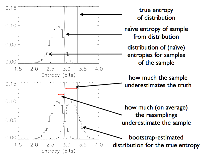
The symbols are nice, but as is usually the case, a picture helps to build intuition. Instead of going through a lot of effort to make my own figure, I stole Figure 1 from DeDeo's paper (see page 2249)⁴:

The solid vertical line is the true entropy, what I've been calling $H(\mathbf{p})$. The dashed line is the plug-in estimate of the entropy, $\hat{H} = H(\hat{\mathbf{p}})$. The histogram in the top panel is the estimated distribution using the bootstrap samples $\{ \hat{H}^{b}\}_{b = 1}^{B}$. How far away the average of this distribution is from the estimated entropy gives us a guess at how far our estimated entropy is from the true entropy. Sometimes it seems like turtles all of the way down, but in reality this technique works.

DeDeo, et al., have a Python package that implements their bootstrapped entropy estimator, amongst others. They called it THOTH. From DeDeo's site: "THOTH is named, playfully, after the Ancient Egyptian deity. Thoth was credited with the invention of symbolic representation, and his tasks included judgement, arbitration, and decision-making among both mortals and gods, making him a particularly appropriate namesake for the study of information in both the natural and social worlds."

There's still no final word on the appropriate way to estimate entropy. We've seen three: the maximum likelihood estimator, the Miller-Madow estimator, and the bootstrap estimator. Each of them have their strengths and weaknesses, and will work or fail in different situations.

As a final aside, this has not been a purely academic⁵ exercise for me. I've been performing mutual information and informational coherence estimation for joint distributions with very large alphabets in the hopes of detecting dynamical and computational communities in social networks⁶. In these cases, it becomes important to deal with the biases inherent in estimating entropies, since with limited sample sizes, the biases in these estimators seem to indicate much higher mutual information / informational coherence than is actually present. This is bad when you're trying to define functional communities.

Just another example of how careful we have to be when dealing with information theoretic analyses.

Which explains the name 'bootstrap,' at least if you're familiar with early 20th century turns of phrase: we've managed to answer our question (what is the sampling distribution of our estimator) without any extra help.↩
And by the Glivenko-Cantelli Theorem (aka. the Fundamental Theorem of Statistics), it almost surely will.↩
Which is unfortunate, because on page 130 of An Introduction to the Bootstrap, Brad and Rob give a very simple twist on the bootstrap estimator of bias which gives much better convergence results. I'm not completely sure the twist applies to the case DeDeo considers (since typically Brad and Rob are concerned with data from a continuous distribution where data points will never repeat), but if it does, then the change to DeDeo's code should be trivial. Something to look into.↩
Which, to be honest, I didn't fully grasp at my first pass. Without the math, it's hard to get the bootstrapping entropy idea across. Hopefully with the combination of the two, things make a little more sense.↩
Well, depending on ones definition of academic.↩
This will all hopefully show up in a paper in the near to medium future.↩

Analyzing and Bootstrapping Our Way to a Better Entropy Estimator — Part I, Analytical

First, the analytical way to get at a better entropy estimator. As we saw in the previous post, it's known that any estimator of the entropy of a discrete distribution will be biased. And it's also known that the maximum likelihood estimator, while biased, is in some way the 'best' estimator (at least for large sample sizes) in that it's the minimax estimator for entropy. So, it might make sense to see if we can patch up the maximum likelihood estimator by trying to account for its bias.

The way to go about this is, what else, a Taylor expansion. Again, Liam Paninski has already done most of the work for us. But let's try and demystify parts of his derivation, which in my opinion goes a little too far off the pure math deep end (though I'm sure he had good reasons for doing so that didn't make it into the paper proper).

We want to make a statement about the bias of the maximum likelihood estimator for entropy $\hat{H} = H\left(\hat{\mathbf{p}}\right)$, where $H$ is the usual entropy functional of a probability vector $\mathbf{p} = (p_{1}, \ldots, p_{d})$, \[ H(\mathbf{p}) = -\sum_{j = 1}^{d} p_{j} \log p_{j}.\] (Logs will be taken base-$e$, mostly for convenience. We can always convert from nats to bits at the end.) This means we need to know the expected value of $\hat{H}$. We could try to compute this directly, but remember that the expectation is taken over the sample $(X_{1}, \ldots, X_{n})$ used to compute $\hat{\mathbf{p}}$, and we don't want to assume any particular distribution for the $X_{i}$ (this is why the estimator is 'non-parametric'). Instead, we'll use a (multi-dimensional) Taylor expansion of $\hat{H}$ about the true $\mathbf{p}$, and hope that the linear approximation holds when $\hat{\mathbf{p}}$ is close enough to $\mathbf{p}$. The result looks nasty¹, but the intuition is simple, and we already saw how to do this for a scalar function of two variables. The linear expansion is the same as for a scalar function $f$, \[ f(x) = f(x^{*}) + (x - x^{*}) f'(x^{*}) + r(x, x^{*}),\] with the scalar derivative $f'$ replaced by the gradient. Thus, we expand the entropy functional² as \[ \hat{H} = H(\mathbf{p}) + (\hat{\mathbf{p}} - \mathbf{p})^{T} (\nabla H) (\mathbf{p}) + r(\hat{\mathbf{p}}, \mathbf{p})\] where \[ ((\nabla H) (\mathbf{p}))_{j} = - (\log p_{j} + 1).\] You can carry this through (at this point, it's an exercise in dot products and basic facts about probability mass functions), and you'll find that \[ \hat{H} - H(\mathbf{p}) = - D_{KL}(\hat{\mathbf{p}} || \mathbf{p}),\] where $D_{KL}(\mathbf{q} || \mathbf{p})$ is the Kullback-Leibler divergence, \[ D_{KL}(\mathbf{q} || \mathbf{p}) = \sum_{j = 1}^{d} q_{j} \log \frac{q_{j}}{p_{j}}.\] As Paninski points out, this is another nice way to see that the maximum likelihood estimator is negatively biased, since one of the properties of the Kullback-Leibler divergence is that it's always non-negative, so the expected value of $- D_{KL}(\hat{\mathbf{p}} || \mathbf{p})$ (and hence the bias) must be non-positive.

With a lot more work (Taylor expand the Kullback-Leilber divergence, etc.) that I will skip, you can show that the bias is given by \[ \text{Bias}(\hat{H}) = E[\hat{H}] - H = - \frac{d - 1}{2 n} + O(n^{-2}).\] Thus, the leading order term in the bias depends on the alphabet size $d$ and the sample size $n$, and decreases like $n^{-1}$ for large $n$.

Since we know that this is the (approximate) finite-sample bias of the maximum likelihood estimator, it follows that \[ E[\hat{H}] + \frac{d - 1}{2 n} \approx H,\] which motivates a new estimator, the Miller-Madow estimator, \[ \hat{H}_{MM} = \hat{H} + \frac{\hat{d} - 1}{2 n}\] which is approximately unbiased. Note that we had to include another estimator, $\hat{d}$, in our estimator. This is because we don't necessarily know, a priori, the alphabet size, and have to estimate it from the number of symbols we see in the data. Take, for instance, corpus analysis of texts, where we use a 'bag of words' model. What is the number of words in the English language? I doubt we know this number exactly.

This estimator is nice, because it's very simple. Our analytical derivation has done all of the work up front, and all we have to do is add on the $\frac{\hat{d} - 1}{2 n}$ term to our naive estimator, and we're already better off. The Miller-Madow estimator is frequently used as a straw man model, at least in the papers I've read about entropy estimation.

In Part II of this 'series,' we'll look at a different estimator, the bootstrap entropy estimator, that, like all bootstrap estimators, requires computational work on each go. This approach (letting the computer do the heavy lifting) has the advantage that we don't have to think very hard, and turns out to work very well in practice.

One of my undergraduate mathematics professors told us a story about how a colleague of his was paid a large sum of money for photocopying the multidimensional Taylor's theorem. In truth, given the context of the story (financial mathematics), I think he photocopied the result for Ito's Lemma. Wikipedia has certainly ruined the monopoly that mathematicians have over theorems.↩
This is where Paninski gets a little too math-y for my tastes. He claims we need to use a Frechet derivative here, which generalizes the usual derivative we're used to. To my eyes, $H$ doesn't require this machinery: it's just a scalar function of $\mathbf{p}$.↩

Mathematical Limits

A comment I often here from non-mathematicians in the sciences: "I wish I had learned more mathematics."¹ This is usually followed by a story about how they realized that math shows up a lot more often than they'd thought, compared to their initial training, in their discipline.

Fortunately, I didn't have this problem. I continued to take mathematics courses in college past the usual stopping point for science majors (which, for some reason, is Calculus II, as if that's the apex of mathematics²), mostly thanks to this man. At first he encouraged me to take discrete mathematics, then linear algebra, and at that point I was hooked. He got me through the door to see that mathematics is more than just computing integrals and derivatives.

While I did take more mathematics courses than the usual science major (I did, after all, end up majoring in math, after switching from chemistry), I did not take more mathematics courses than the usual mathematics major. I have never had a course in complex analysis, partial differential equations, topology, number theory, or 'advanced' analysis (i.e. measure theory).

Which makes me wonder: how far will I get in my career before I begin to say, "I wish I had learned more mathematics!"

I know enough about a lot of mathematical topics to speak roughly about them. I have an intuition about the Lebesgue measure (chop up the range instead of the domain), and can spout off that a Banach space is a complete normed vector space. And I've certainly heard enough about certain mathematical topics to know I should know more about them. It's a running joke with my housemates that they should run a directed reading program (something usually for undergraduates) to teach me measure theory.

But on the flip side of the coin, I've seen how far people can get without knowing the finer details of the mathematics underlying their field (a lot of physicists working in essentially stochastic processes who don't know measure theory, for example, or computer scientists working in machine learning who don't really have a firm background in elementary probability theory). For the record, I think this is bad, but I also think that these people publish more than I do and currently have a bigger impact than I do, so I should pay attention to this.

Of course, this entire discussion is a little silly. It's not as if I can't continue to learn more math³. My education didn't stop when I finished taking courses⁴. I'm more or less self-taught in modern statistics, except for what I learned in undergrad from Roger Coleman. This indicates that with enough time and attention, I should be able to teach myself about other subject as well.

There's no doubt in my mind that knowing more math can only help me. But I only have a finite amount of time on this planet, and a finite amount of focus in any given day, so I have to pick and choose the things that I spend time learning. That means, from any given discipline, I can only go so deep⁵. How deeply do I need to go into mathematics? I probably should learn the rudiments of measure theory. I probably don't need to learn much category theory.

I don't think there's a 'correct' answer to this question. Different computational scientists will have differing success with differing degrees of mathematical education. I guess what it comes down to is what I want. And what I want is to continue learning mathematics.

Now if I could just convince myself of that.

A comment I often here from non-mathematicians outside of the sciences: "Math? What can you do with that?" Clearly these people have never seen the show Numb3rs.↩
To quote John Cook, "If calculus students think they're near the vanguard of math, they're off by 300 years."↩
It sounds hokey, but I really think I 'learned how to learn' in graduate school. To quote Mark Reid, "[learning mathematics] involves sitting alone in a room being confused almost all the time." Graduate school teaches you to push through this confusion and reach the understanding on the other side.↩
Though self-directed learning is hard. Not only because the more advanced material is more difficult, but also because I have to find the motivation to sit down and teach myself something. Even if I really want to learn the subject, this can be more difficult than it should be.↩
In physics, for instance, I would like to formally study statistical mechanics. Probably from this book.↩

Delta, Taylor, and Physical Chemistry — How do errors propogate?

I took Physical Chemistry my junior year of undergrad¹, basically a watered down course in classical thermodynamics with a modicum of statistical mechanics. The lecture portion of the course was fantastic. The lab portion, less so. (There's a reason I become a computational scientist.) We spent hours measuring out reagents, timing reactions, and computing equilibrium constants. Why we did all of those things are beyond me. I think mostly to learn about proper lab technique.

After we finished up in the wet lab, the next step was to write up a lab report. For your general amusement, here's an example report on the chemical kinetics of the reaction between 2,4-dinitrochlorobenzene and piperidine². I hated writing those, as I now hate writing journal articles.

As a part of the lab writing process, though not in the lab above, we had to do this terrible thing called 'propagation of errors.' Since we're fallen beings and our instruments are faulty, we worry about the inaccuracies in our measurements. We usually have some idea about how inaccurate our measurements are. The lore goes something like this: if you have a ruler that only measures to the nearest millimeter, you're uncertainty in the measurement is around 0.5 millimeters. However, we would also like to derive things from our measurements. (We are trying to do science after all, and not big data.) And thus, we need to have some idea about how uncertain we should be about our derived quantities.

And this is where propagation of errors comes in. At the time (a mere seven years ago), propagation of error formulas seemed like the sort of thing best left to tables. How could anyone derive these themselves? I had vague notions that the formulas seemed a lot like partial derivative formulas I'd seen in multivariate calculus (just a semester before), with some squares thrown in, but couldn't see a connection beyond that. Years would pass.

And then I trained to become a passable mathematician and statistician. Now I know my intuition about partial derivatives was correct, and the missing ingredient was a bit of probability theory. (Again: how probability theory doesn't get taught to students of the hard sciences in a formal manor is beyond me. We have to get past teaching statistics only in lab methods courses and start giving Kolmogorov, et al their due.)

Here's the setup³. We have two quantities, call them $X$ and $Y$, that we measure. These might be the voltage and current in a circuit, where we're interested in computing the resistance⁴. We'll treat these as random variables. Again, we are fallen beings in an imperfect world. And probably a bit hung over from that party the night before. As such, we need to specify things like means and variances for the random variables. Since we typically only measure something a single time in a chemistry lab, we'll take the mean values to be the measured values (why not?), and the variances to be our instrument capacities (the 0.5 mm in a 1-mm demarcated ruler). What we really want is to know the uncertainty (i.e. variance) in $Z = g(X, Y)$, our observed quantity. Again, in the electrical example, we might compute $R = g(V, I) = \frac{V}{I}$, and want to say something about how certain we are about the resistance.

How can we do this, using only our knowledge about $g$ and the variances of $X$ and $Y$? A Taylor expansion, of course! Recall that a smooth function of two variables looks more or less like a plane if we get close enough to its surface. Thus, we can write out a linear approximation (truncating the Taylor expansion at the linear term) of $g$ about the mean values of X and Y as \[ Z = g(X,Y) \approx g(\mu_{X}, \mu_{Y}) + (X - \mu_{X})\frac{\partial g}{\partial X}(\mu_{X}) + (Y - \mu_{Y})\frac{\partial g}{\partial Y}(\mu_{Y}).\] We now have written $Z$ as an affine transformation of $X$ and $Y$. And variances behave very nicely with respect to affine transformations. In particular, \[ \text{Var}\left(a + \sum_{j = 1}^{p} b_{j} X_{j}\right) = \sum_{j = 1}^{p} b_{j}^{2} \text{Var}(X_{j}) + 2 \sum_{i < j} b_{i} b_{j}\text{Cov}(X_{i}, X_{j}).\] (We could wrap this all up very nicely using linear algebra into a quadratic form. But that's likely to scare the chemistry majors. Heck, it scared me in my senior year mathematical statistics class.) Applying this to our linear approximation of $Z = g(X, Y)$, we get that \[ \text{Var}(Z) \approx \left(\frac{\partial g}{\partial X}(\mu_{X})\right)^{2} \text{Var}(X) + \left(\frac{\partial g}{\partial Y}(\mu_{Y})\right)^{2} \text{Var}(Y) + 2 \text{Cov}(X, Y) \frac{\partial g}{\partial X}(\mu_{X}) \frac{\partial g}{\partial Y}(\mu_{Y}).\] Typically, we don't have any reason to believe that the errors in $X$ and $Y$ are correlated, say, if we've measured them with two different instruments⁵, so the covariance term drops and our expansion is just in terms of the weighted variances (weighting by the squared partial derivatives) of $X$ and $Y$. From this point, it's easy enough to compute the propagation of errors formula for an arbitrary $g$. Though of course we must always keep in mind that we've made two approximations. First, we've truncated the Taylor expansion of $g$ at the linear terms. Second, we're ultimately substituting in our measured values of $X$ and $Y$ for $\mu_{X}$ and $\mu_{Y}$. Typically, these approximation errors are overwhelmed by stochastic errors (i.e. measurement noise). Besides, what else are we to do?

This is all related to something statistician's call the delta method. The delta method considers the limiting distribution of the transformation of a random variable whose own limiting distribution is known to be normal. The intuition is relatively straightforward: if $X$ is normal, then $a X + b$ is also normal (normal random variables live in the stable family of distributions). Thus, if we have a transformation $g$ that is almost linear, then $g(X) \approx a X + b $ for some $a$ and $b$, and thus $g(X)$ should have an approximately normal distribution. Recall that our Taylor expansion is taken about the mean value of $X$. Thus, if $X$ spends most of it's time around $\mu_{X}$, the approximation will be very good, and the normal approximation will good. Proving this result takes a decent amount of algebraic manipulations, and can be found in Larry Wasserman's All of Statistics.

The delta method comes in handy when dealing with maximum likelihood estimators for distributions that satisfy certain regularity (i.e. smoothness) assumptions. In these cases, we know that $\hat{\theta}$ is asymptotically normal, and thus $g\left(\hat{\theta}\right)$ will also be asymptotically normal (given a few assumptions on $g$). Like usual, the Taylor expansion has saved us a great deal of work, both in terms of theory and computation.

Looking over the laboratory textbook we used in Physical Chemistry, I am surprised by how much more probability theory and statistical theory is present than I remember. I suppose I didn't have ears to hear at the time (I thought I hated statistics), and didn't have eyes to see (i.e. I didn't have the requisite background for any of the material to make sense). But that said, this textbook doesn't even hint at the derivation of the propagation of errors formula. Apparently linear approximations are above and beyond what a standard undergraduate taking a physical chemistry course is expected to know. (Which is outrageous.)

A youthful folly, thinking I'd be a chemist like my father and brother.↩
But seriously, I used to do this stuff?!↩
What follows largely borrows from here.↩
Presumably to confirm Ohm's law. Again.↩
Of course, we always run the risk that all measurements are made by the same person. If I happened to be your lab partner, this was something you had to worry about.↩

Medical Diagnostics

I went to the cardiologist today for a followup on a previous visit and stress test echocardiogram. The verdict from the stress test: my heart pumps fine. (This is, perhaps, unsurprising. I'm relatively young, my family has no history of heart disease, and I lead a moderately healthy lifestyle.) Which is reassuring. But my symptoms still remain: shortness of breath, heart palpitations, fatigue after eating, etc.

This has been my first personal experience with the medical establishment. I managed to stay away from doctors for the first 25 years of my life, except for the occasional mandatory check up. And I preferred it that way. Overall, the experience with the doctors has been pleasant enough, once I learned that specialists require scheduling appointments months in advance and an 8:45am appointment time means I'll be seen at 10:15am.

Overall, I wish I could have a more intellectually fruitful conversation with the doctors and nurses¹. As an example: an echo technician asked me what my 'typical' blood pressure is. I told him 120 over 80. He laughed, since that is the standard healthy blood pressure. I, on the other hand, don't know what to answer. Blood pressure is naturally variable. As someone trained in statistics, I don't think it's honest to give a single number. And if I must, why not give the 'healthy' value. Here's my blood pressure over the past 70 days:

Each point corresponds to the average of three blood pressure readings taken over a ten minute period (thus, even this plot masks the variability inherent in blood pressure over small time windows), alternating morning and evening. The blue curve is a LOESS fit with the default smoothing parameter (I can't begin to imagine explaining $k$-fold cross validation...), mostly to guide the eye. Clearly, my systolic blood pressure (the larger number) has been declining, while my diastolic (the smaller number) increased for a bit and is now on the decline². This change can be explained by my trip to Santa Fe: blood pressure tends to increase at higher altitudes.

So, what was I supposed to say for my 'typical' blood pressure, again?

I understand that medical doctors have a specific set of skills and knowledge. Skills and knowledge I can't even begin to claim. (I still have trouble distinguishing between my shoulders and my elbows. I keep thinking I should learn some basic anatomy and physiology. They've been added to the long list of topics I want to study but probably never will.) But it seems like, at least so far, diagnostic medicine is stuck in the dark ages. Which is why I welcome our robot overlords.

It's funny (though perhaps not strange) that none of my complaints center around the usual things one hears about medicine. Probably because I'm currently covered by my parents' health insurance (until September, when I'll be too old for that), and have enough saved up to deal with these sorts of rainy day expenses. Honestly, I'd be much happier paying anything if I felt like medicine were practiced more like physics and less like haruspicy.

I know I'm being too harsh on diagnostic medicine. I've seen too many episodes of House and read too many futuristic books about the biomedical singularity for my own good. I think that someday medicine will meet the expectations I have currently set for it. But today is not that day.

This is partially my fault. I definitely suffer from the white coat effect: doctors seems so confident when they talk to me, and I question any nagging concerns I have as hyperchondria. I also suffer from white coat phenomenon: my blood pressure tends to read in the high range at the doctor's office, even though at home it reads well within the healthy range.↩
One positive thing that has come out of this experience: I've begun to learn some of the physiology-related lingo. The dark side of this: long stretches of time spent on WebMD and health-related message boards.↩

How many ways can you estimate entropy?

I've written a good deal about entropy . But in all that time, I haven't talked about the easiest (though still hard) problem of how to estimate discrete entropy. (See older posts for how to estimate differential entropy.)

As a refresher, for a discrete random variable $X$ with support $\mathcal{X}$ and probability mass function $p(x) = P(X = x)$, we define the Shannon entropy as \[ H[X] = -E[log_{2} p(X)] = -\sum_{x \in \mathcal{X}} p(x) \log_{2} p(x).\] This is a 'population level' value. You can think of it as a parameter of the distribution, something akin to the number of yes-no questions to identify the value of $X$ upon each new realization you come across.

Of course, in the real world, we often observe a sample from $P_{X}$, namely $X_{1}, \ldots, X_{n}$ and want to say something about the distribution that generated that sample. That is, we want to do statistical inference: to make guesses at this uncertainty parameter.

How many different ways can you estimate the entropy of a distribution from a sample? It turns out: a lot¹. And researchers are still inventing new ones.

The simplest way to estimate the entropy is to use a naive / plug-in / non-parametric / maximum likelihood estimate². All of these mean to do the thing you (or at least I) would most naturally do. Estimate each of the probabilities $p(x)$ as the proportion of your sample that took the value $x$, call these $\{\hat{p}(x)\}_{x \in \mathcal{\hat{X}}}$, and compute

\[ \hat{H} = -\sum_{x \in \mathcal{\hat{X}}} \hat{p}(x) \log_{2} \hat{p}(x).\]

This seems like a reasonable enough way to go about the problem. But it turns out the estimator is biased for any finite $n$, though asymptotically unbiased in the limit as $n \to \infty$. We can show this relatively easily by applying Jensen's inequality. Jensen's inequality tells us the result of exchanging expectations with function evaluations. In particular, for a concave function like entropy, we have that \[ E[f(X)] \leq f(E[X]).\] What do I mean by entropy being concave? If we consider entropy to be a function of $\mathbf{p} = \{ p(x) \}_{x \in \mathcal{X}}$ (that is, think of the probabilities as a vector), then we can clearly think of $H[X]$ as a (multi-dimensional) function $H(\mathbf{p})$ taking this vector as an input. Entropy turns out to be concave in $\mathbf{p}$ (i.e. you can prove this), and as such we have that \[ E[H(\hat{\mathbf{p}})] \leq H(E[\hat{\mathbf{p}}]) = H(\mathbf{p}) = H[X].\] We have then that the bias is \[ \text{Bias}(\hat{H}) = E[\hat{H}] - H \leq 0,\] so our naive estimator will always be negatively³ biased.

The fact that our estimate of entropy is biased sounds worrisome. But it shouldn't worry us too much, since in fact any estimator we could come up with for the entropy of a distribution will be biased. See page 1236 of Paninski's Estimation of Entropy and Mutual Information for a slick proof. Thus, all we can do is attempt to mitigate⁴ the bias, but we can never hope to remove it completely.

In a future post, I'll discuss two methods for dealing with the bias, one very old, the other much more recent.

Because I can't leave a blog post like this without showing a few plots, here's a simple application of entropy estimation. Consider a probability distribution with the probability mass function \[ P(W = w) = C \, w^{-1}, W = 1, \ldots, 50\] where $C = \left(\sum\limits_{w = 1}^{50} w^{-1}\right)^{-1}.$ This distribution is within the Zipfian family⁵, and is a popular statistical model of, for instance, frequency of words in a document. (Hence the choice of $W$ for the random variable.) The distribution itself looks like this:

with some of the words getting much of the probability mass, and many getting only a little (the 'long tail' of the distribution, though not so long as most, since it has finite support).

We can estimate the entropy of the distribution for varying sample sizes $N$, and we know the true entropy of the distribution is approximately 4.612478:

All of our estimators converge on the truth (except for the Bayesian one, but, well, it's Bayesian) as the sample size increases. I'll talk about two of these estimators ('MM', which stands for Miller-Madow, and 'Bootstrap') in a future post. Both clearly do better than the naive estimator, and the Miller-Madow estimator for a simple reason, and the bootstrap for a very clever reason.

This turns out to be one of those methodological problems that I've been 'doing wrong' for a while now. I didn't realize how subtle entropy estimation is. But now (I hope), I have a basic understanding of some of the intricacies. And hopefully can leave the follies of my youth behind.↩
Non-parametric because we're treating the distribution as a categorical random variable, instead of specifying any particular distribution like Poisson, binomial, etc. If we did have reason to assume a parametric model, we'd be better off estimating the parameter instead of estimating each of the individual probabilities. Parametric models are nice, when they're well-specified.↩
Mind you, this doesn't mean any given estimate will be less than the true entropy of the distribution. That would be nice. This statement only says the expected value of the sampling distribution will always be less than true value. Any given realization from the sampling distribution can lie on either side. As usual, we have to be careful in our thinking about statements regarding the sampling distribution.↩
Always keeping in mind the bias-variance tradeoff. Classical statistics worried about finding minimum variance unbiased estimators (abbreviated MVUE). (See the wonderful theory wrapped up in the Cramér-Rao.) But we might be able to find slightly biased estimators with much better variance that give us an overall smaller mean-squared error. Most of the work I've seen on entropy estimation focuses on minimizing the bias, but many do implicitly account for the variance by computing mean-squared error. This is good, because an unbiased estimator is no good if the actual estimates are scattered far away from the true value.↩
A power law, for those who care about such things. Personally, after spending a month in Santa Fe, I'm sick and tired of hearing about power laws.↩

Non-Ergodic Economics — Or, Multiplicative Games are Bad

Here's a simple game, motivated by a talk by Ole Peters. Suppose we start with $R_{0}$ dollars. We flip a fair coin, and on each flip of the coin, we win 50% if the coin comes up heads, and lose 40% if the coin comes up tails. This sounds like a good game: on the first flip, our expected winnings are \[ \frac{1}{2} 1.5 R_{0} + \frac{1}{2} 0.6 R_{0} = 1.05 R_{0},\] so it looks like we'll do well. But now, as Peters puts it, lets add in a dynamic: let's see if we want to keep playing this game. This seems like a reasonable thing to do, since when people invest, they don't tend to put their money into the stock market for a day and then pull it out.

In this case, we have ourselves a stochastic process $\{R_{t}\}_{t = 0}^{\infty}$ where $R_{t}$ is the amount of money we have after $t$ time steps. It's clear from the description of the game that the process will evolve according to \[R_{t} = \left\{\begin{array}{cc} 1.5 R_{t-1} &: \text{with probability } \frac{1}{2} \\ 0.6 R_{t-1} &: \text{with probability } \frac{1}{2} \end{array}\right.\] This is a nice way to look at the process procedurally (for instance, it shows us the process is Markov, and gives us an easy way to simulate from it). But it will get unwieldy if we want to do anything analytical. Instead, notice that to determine $R_{t}$, we are flipping a coin $t$ times, and counting up the number of heads and tails¹, which tells us how many times we need to multiply $R_{0}$ by either 1.5 or 0.6, respectively. Coin flips are governed by the binomial distribution, and we are multiplying, so this stochastic process is called the binomial multiplicative process². After $t$ flips, the only values that $R_{t}$ can take are $R_{0} 1.5^{i} 0.6^{t-i}$, $i = 0, \ldots, t$, since we can have had zero heads, one heads, two heads, ..., up to $t$ heads, and it takes those values with probability $\binom{t}{i} \left(\frac{1}{2}\right)^{i} \left(\frac{1}{2}\right)^{t - i} = \binom{t}{i} \left(\frac{1}{2}\right)^{t}$. Thus, we've fully specified the distribution of the process for any length of time, and, in principle, we're done. For example, if we want to compute the mean of the process, we group terms and apply the binomial theorem, giving us \[ m(t) = E[R_{t}] = R_{0} 1.05^{t}.\] Thus, over time, the expected value grows exponentially. This again makes it seem like we want to play the game. Finally, we can compute the variance as a function of time, giving us \[ V(t) = \text{Var}(R_{t}) = R_{0} (1.305^{t} - 1.1025^{t}),\] which again increases with time. (This is our first sign that perhaps we don't want to play the game, if the winnings of people get more and more spread out as the game goes on.) We can plot both $m(t)$ and $V(t)$ as a function of time,

for the mean and

for the variance. The black dots were computed using a sample of ten thousand players. The red dots are the analytical values. As anticipated, we get good agreement between the sample values and the population values. Finally, note that the plots are semi-log. This is commonly done without mention. But I think it's worth mentioning.

So far, we've looked at measures of center and variation. But again, we have the entire distribution available to us, so why not use it? Let's look at the distribution of wealths for a society of people playing this game. First, here's a schematic of how the game plays out: This looks very much like a (biased) random walk, and for good reason: if we take the logarithm of a multiplicative process, it becomes an additive process, and we in fact find ourselves with a random walk. This explains the use of logarithms throughout. Logarithms also makes the computer much happier. If we shaded the lines in by the number of sample paths that traverse them, we would see that most people follow along the central trajectory, with less and less people following along the further out branches. (We see this explicitly in the most extreme trajectories, which don't get traced out with only 10000 sample paths.) We can of course compute the proportion of walks that end up at node, first for $t = 1$

and then for $t = 10$

Again, not that the x-axis is scaled to have logarithmic spacing. As expected, this gives us a binomial distributions. Recalling that a binomial process (a series of fair coin flips!) underlies the dynamics we observe, this shouldn't be too surprising. What we do see is that most people have very little money ($50 or less), while a few people have much more money ($5000). If we keep playing this game out to, say, $t = 1000$, we see

In this case, most people have $$1.322 \times 10^{-23}$ or less, while a few have $$1.233841 \times 10^{176}$, an astronomical amount of money. This explains the strange discrepancy we've seen between the expected value as a function of time (which continues to increase), and what Peters points out at the beginning of his lectures (and I have so far failed to do), namely that any particular person is very likely to lose a great deal of money if they keep playing this game. In particular, here's a single realization played out over the course of 10000 goes at the game:

This person has clearly lost out. And they are the norm. Another reminder that average values don't necessarily capture what you would like to know about a distribution.

Since scalar multiplication is commutative, it doesn't matter what order the heads and tails occurred.↩
Ole only gave this name in passing during his lecture. Again, I've noticed that mathematicians don't feel comfortable with something until it has a name, while physicists don't seem to mind.↩

Back to Reality

I returned to the East coast today after spending a month in New Mexico at the Santa Fe Institute's Complex Systems Summer School.

The school was a fantastic experience, and I highly recommend it.

Some things I learned, in no particular order:

Asking interesting questions is sometimes more important than having a method on hand to answer them.
Old habits die hard. A speaker would admonish us not to do something, and within the next week, we would see someone doing precisely that thing.
Complex systems is a field defined largely by its questions, not its techniques. Though some techniques stand out: agent-based models (really, a generalization of cellular automata), nonlinear dynamical analyses of systems (either through modeling or time series methods), networks (a topic du jour this summer)
Not many statisticians were present at the summer school, as participants or lecturers. With a few important exceptions. This is strange, since statisticians, almost by definition, study complex systems.
Interests vary widely. We had several lectures on ecology that I couldn't follow, despite the speakers best efforts. Mostly because I have very little interest in ecology. I imagine the ecologists in the crowd felt similarly about lectures on the mini-max optimality of kernel methods for non-parametric regression.
When can one begin to call oneself a physicist / biologist / computer scientist / mathematician / economist / etc.? Mostly, we all self-identified as one of these (or many other) specialties. But I still feel uncomfortable introducing myself as a mathematician in a non-specialized academic setting. I don't want people to get the misimpression that I have a firm understanding of measure theory, for example.
This is a multinational field. I met more non-US researchers this summer than I have in my entire life. Many of the researchers from Europe are earning PhDs specifically in Complex Systems Science. We have far fewer such degrees in the US. It's interesting to see Europe beat out the 'New World' in this regard.
Physicists, especially former particle physicists, dominate the Institute's ranks. Which is interesting, since I have so very little interest in fundamental physics. I agree with Sean Carroll that the physics underlying the everyday world is largely understood. This is a risky claim to make. Physicists at the end of the 19th century made similar claims. But this time we're right? Anyway, physicists are great at entering a field, equations blazing, and coming out intact.
I can no longer distinguish age groups. If you're over 22, I probably think you're in your mid to late 20s. I imagine that assumption will grow linearly with my own age.
Santa Fe is blessed with beautiful weather, sans the drought. Climate change is no fun for forest fires.

Well, that's it. I may reflect more on the experience when I'm less tired. This will have to do for now.