All I Really Need for Data Analysis I Learned in Kindergarten — Venn, Shannon, and Independence
Venn1 diagrams are one of the first graphical heuristics we learn about in elementary (middle? high?) school. They're a convenient way to represent sets2, and allow for the easy visualization of set operations like intersection and union.
Once we have sets, we can consider a measure3 on top of those sets, and we have ourselves the beginnings of measure theory. And thanks to our good friend Andrey Kolmogorov, we can then employ them in probability theory, which is really nothing but measure theory restricted to a space with measure 1.
Elementary probability theory was my first formal introduction to the usefulness of Venn diagrams. If you have two events \(A\) and \(B\), and want to talk about probabilities associated with them, you can draw a general two-circle Venn diagram,
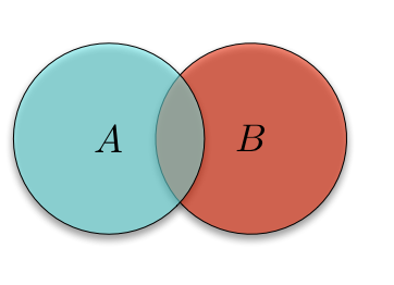
and use that diagram to get out any quantity involving intersections and unions4. For example, the probability that \(A\) or \(B\) occurs is the probability \(P(A \cup B)\), which we see is just the 'area' of the union of the two sets. Similarly, the probability that \(A\) and \(B\) occur \(P(A \cap B)\) is the area of the intersection of \(A\) and \(B\), which we can get by computing \(P(A) + P(B) - P(A \cup B)\).
This is all old news, and common fair for any introductory probability course. But as I said in one of the footnotes, these sorts of Venn diagrams can't represent any sort of conditional probability, which we're often interested. A common pitfall of a beginning probabilist is to think that disjointness means independence5. Recall that two events \(A\) and \(B\), both with probability greater than 0, are independent if
\[ P(A \cap B) = P(A) P(B) \]
or equivalently if
\[ P(A | B) = P(A) \]
or
\[ P(B | A) = P(B). \]
In words, this means that two events are independent if the probability of one occurring doesn't depend on the other occurring. This seems like a reasonable enough definition. But what about when two events are disjoint? Are they independent?
If two events are disjoint, then \(P(A \cap B) = 0\). But, with some manipulation, we see
\[ P(A | B) = \frac{P(A \cap B)}{P(B)} = 0 \neq P(A), \]
since we assumed that \(P(A) > 0\). Thus, \(A\) is not independent of \(B\). In fact, they're as dependent as they could get: once we know that \(A\) happens, we know for sure that \(B\) did not happen.
I found this result so striking that, at one point during a intermediate probability theory course, I wrote in my notebook, "There is no way to show independence with Venn diagrams!" It seems like we should be able to, but remember that Venn diagrams only allow us to show things about intersections and unions, not conditioning.
But I was only part right about this conclusion. It turns out a slightly different sort of Venn diagram6 perfectly captures these conditional relationships. To get there, we need to expand our probabilistic language to include information theory7. For two random variables \(X\) and \(Y\)8, we will specify their joint probability mass function by \(p(x,y)\). Then their joint entropy can be computed as
\[ \begin{align} H[X, Y] &= - E[\log_{2} p(X, Y)] \\ &= -\sum_{(x, y) \in \mathcal{X} \times \mathcal{Y}} p(x, y) \log_{2} p(x,y) \end{align} \]
and their marginal entropies \(H[X]\) and \(H[Y]\) can be computed in the same way using the marginal probability mass functions \(p(x)\) and \(p(y)\). We'll also need two more objects (and a third guest star), namely the conditional entropies \(H[X | Y]\) and \(H[Y | X]\), where the first is defined as
\[ H[X | Y] = -E[\log_{2} p(X | Y)]\]
and the second is defined in the obvious way9.
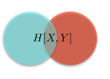
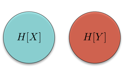
To get the Venn diagram, we start with an empty Venn diagram
![]()
where the circle on the left contains the 'information' in \(X\) and the circle on the right contains the 'information' in \(Y\)10. Thus, it makes sense that if we consider the union of these two circles, we should get the information contained in both \(X\) and \(Y\), namely the joint entropy \(H[X, Y]\), and we do:
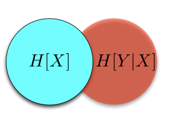
We've already called the circle on the left the information in \(X\), so it makes sense that this should correspond to the entropy of \(X\), \(H[X]\). And it does. But what do we get if we take away information in \(X\) from the information we have about both \(X\) and \(Y\)? As expected, we get the information left in \(Y\) after we've conditioned on \(X\), namely \(H[Y | X]\):
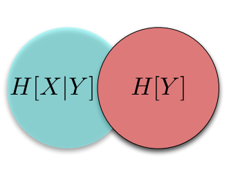
The same results hold if we fix our attention on \(Y\):
The only portion we haven't explicitly named is the portion in the middle: the intersection of the information in \(X\) and the information in \(Y\). This part of the information diagram is called, unsurprisingly, the mutual information between \(X\) and \(Y\), \(I[X; Y]\):
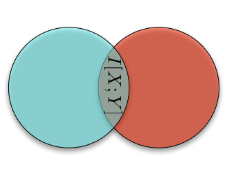
Now we have a name for all of the basic players in elementary information theory, and a way to compute them from each other. For example, the mutual information is
\[ I[X; Y] = H[X] + H[Y] - H[X, Y]. \]
(In the same way that we got \(P(A \cap B)\) above.)
Now we're finally ready to show independence with our new Venn diagram. First, recall a fact: two random variables \(X\) and \(Y\) are independent if and only if their mutual information is zero. This means that two marginal informations in our information diagram have to have zero overlap:
The informations have to be disjoint! (Which is exactly what we mistakenly thought we were getting at with the probability Venn diagrams.)
These information diagrams are nothing new, and have found great success in explicating the properties of stochastic processes in general. Strangely, they only receive the briefest mention in most introductions to information theory11. Hopefully with time, these simple objects from our primary school days will permeate information theory and beyond.
Poor John Venn, who did a lot of work in mathematics, logic, and statistics, mostly gets recalled for his invention of Venn diagrams. As an example of some of his other work: "[Venn] is often said to have invented one of the two basic theories about probability, namely the frequency account. The 'fundamental conception,' he wrote, is that of a series which 'combines individual irregularity with aggregate regularity'." — Ian Hacking, from page 126 of The Taming of Chance↩
At least for three or fewer sets.↩
Where, for the purposes of this post, we'll take 'measure' here literally: think of how you might measure the length, area, volume, etc. of an object. Things are really more complicated, but we'll sweep those complications under the rug for now.↩
But not those properties that involve conditioning. For that, we'll have to introduce a different Venn diagram, as we'll see in a bit.↩
This is yet another case of our everyday language failing to map to the formal language of mathematics.↩
Which, like all things in elementary information theory, may be found in Cover and Thomas's Elements of Information Theory. In this case, on page 22 of the second edition.↩
And start to talk about random variables instead of events. But what is a random variable but another way at looking at an induced probability space?↩
For simplicity, we'll only talk about discrete random variables, i.e. those that take on a countable set of values.↩
The nice thing about information theory is that everything is defined in the 'obvious' way: for whatever quantity you're interested in, compute the expectation of the associated mass function and you're done.↩
We've already seen why it makes sense to talk about 'information' and 'entropy' almost interchangeably, especially for discrete random variables.↩
In the introductory information theory course I sat in on, the professor didn't mention them at all. And as I said, to my knowledge Cover and Thomas only covers them on a single page.↩