Mutual Information for Dynamical Systems
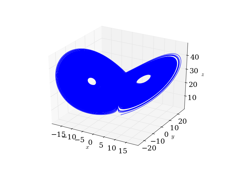
First, the obligatory Lorenz attractor.

Suppose we observe a trajectory from the Lorenz system,
\[ \begin{array}{l} x' &= \sigma (y - x)\\ y' &= x(\rho - z) - y\\ z' &= xy - \beta z \end{array}\]
where we'll set the parameters \((\sigma, \beta, \rho)\) to their canonical values \((10, 8/3, 23).\) We know that this system of differential equations leads to a trajectory \((x(t), y(t), z(t))\) that is chaotic in the usual sense. Since we have the equations of motion, our work is really done.
But suppose instead of having the equations of motion, we only observe the trajectory \((X(t), Y(t), Z(t))\), and only at finitely many points1. (This is what we really have, after all, since I've solved the system of ODEs numerically in time.) A natural question to ask, especially if you don't have the equations of motion, are whether \(X(t)\) and \(Y(t)\) are related. (We really want to know whether all three are related, but these binary questions tend to be easier to handle.)
A common tool for answering these sorts of questions is mutual information. We've already see this quantity before, and we've seen that it is estimable from data alone (if certain assumptions on the underlying process are met). Formally, the mutual information between two random variables \(X\) and \(Y\) (that admit a joint density) is \[ I[X; Y] = \iint_{\mathbb{R}^{2}} f(x, y) \, \log_{2} \frac{f(x,y)}{f(x)f(y)}\, dx\,dy \ \ \ \ \ (*)\] where \(f(x,y)\) is the joint density of the random variables and \(f(x)\) and \(f(y)\) are the corresponding marginal densities.
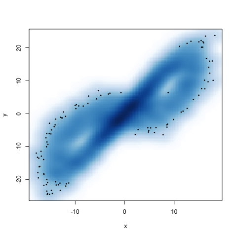
We know that the Lorenz system leads to a chaotic trajectory, so it should hopefully admit a natural measure, and we can hope that measure also has a density. We can get a guess (no proofs from me) at whether this makes sense by looking at the projection of the trajectory onto the \(xy\)-plane, with some smoothing to give us a 2D smoothed histogram:

This is a first pass at the joint density of \(X\) and \(Y\) (really only for visual inspection), and from this figure, it does look like such a thing exists2,3. Basically what we're seeing is that the trajectory fills up the space, but in a very particular way. (We spend more time near the middle of the wings than near the edge of the wings.) In other words, if we didn't know anything about the dynamics, and had to make a guess at where we would be on the trajectory, we should guess we're near the middle.
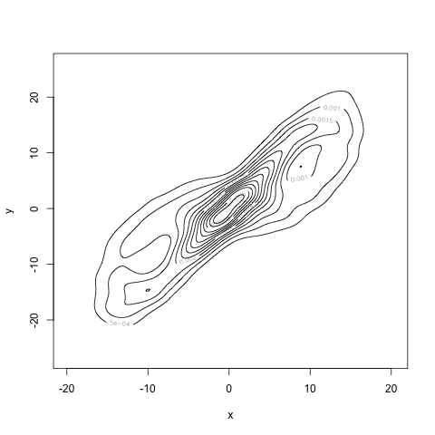
We can more formally estimate the density using kernel density estimators. (Remember that these are the best we can do at estimating a density.) I used bkde2D from R's KernSmooth package4. Here is an estimate with something like 3000 samples from the trajectory, shown as a contour plot.

This is our estimate for \(f(x,y)\), which we'll call \(\hat{f}(x,y)\). As we collect more and more data, this estimate will get closer and closer to the true density. Once we have \(\hat{f}(x,y)\), we can approximate \((*)\), the integral defining mutual information, using quadrature. Of course, now we've introduced two sorts of approximation: (i) approximating \(f\) by \(\hat{f}\) and (ii) approximating the integral by a finite sum. We can reduce the error in the integral as much as we'd like by taking finer and finer partitions of the \(xy\)-space. We're stuck with the error from approximating \(f\) unless we can get more data.
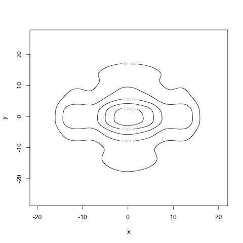
As an interesting illustration, recall that mutual information is, 'in some sense,' measuring the how different the joint density \(f(x,y)\) is from the product of the marginals, \(f(x) f(y)\). Recalling that two continuous random variables are independent if and only if their joint density factors as the product of their marginals, the mutual information tells us how close to independent the two random variables \(X\) and \(Y\) are5. With that in mind, let's look at what the product of the marginals looks like, by marginalizing out the appropriate variables from \(\hat{f}(x, y)\), recalling that \[ f(x) = \int_{\mathbb{R}} f(x, y) \, dy.\] (We can again approximate this integral via quadrature.) If we compute these (approximate) marginals and multiply them, we get the following contour plot for \(\hat{f}(x)\hat{f}(y)\):

This is clearly very different from \(\hat{f}(x,y)\), so we expect the mutual information to take a non-zero value. In fact, when we estimate the mutual information with \((*)\), taking our estimator to be \[ \hat{I}[X; Y] = \iint_{\mathbb{R}^{2}} \hat{f}(x, y) \, \log_{2} \frac{\hat{f}(x,y)}{\hat{f}(x)\hat{f}(y)}\, dx\,dy,\] we find that \(\hat{I}[X; Y] = 1.03.\)
We must keep in mind that \(\hat{I}[X; Y]\) is an estimator for the mutual information, and thus a random variable. It is not the true mutual information. As we collect more data, we should hopefully get closer to the true mutual information. For example, with 100 times as many points, our estimate is \(\hat{I}[X; Y] = 1.40.\) This estimate will bounce around as we collect more data, but hopefully will converge to something in the limit. (I think proving the consistency of our estimator for \(I[X; Y]\) may be tricky. But I also have to believe it's something that a statistician somewhere has spent time pondering.)
I've transitioned from lower case letters to upper case letters to emphasize that now we're considering the trajectory as a stochastic process. We do this for three reasons: (i) it allows us to bring probability theory to bear, (ii) chaotic systems can appear like random processes viewed under the correct light, and (iii) in reality, we usually have experimental noise in any system we measure.↩
People have gone looking for, and found, the density induced by the natural measure for the Lorenz system. Their methodology is much more sophisticated than mine.↩
To fully understand the system, we really want the joint density of \(X\), \(Y\), and \(Z\), namely \(f(x,y,z)\). By projecting into the \(xy\)-plane, we've 'marginalized' out \(Z\), giving us the joint density of \(X\) and \(Y\), \(f(x,y)\).↩
I'm skipping over the important details of choosing the bandwidths for the kernel estimator. There are rigorous ways of doing so. See, for instance, page 316 of Larry Wasserman's All of Statistics.↩
Compare this to correlation, everyone's favorite linear measure of dependence. If two random variables are independent, then their correlation is zero. The converse need not be true.↩