Bridging Discrete and Differential Entropy
For a discrete random variable \(X\) (a random variable whose range \(\mathcal{X}\) is countable) with probability mass function \(p(x) = P(X = x)\), we can define the (Shannon or discrete) entropy of the random variable as \[ H[X] = -E[\log_{2} p(X)] = - \sum_{x \in \mathcal{X}} p(x) \log_{2} p(x).\] That is, the entropy of the random variable is the expected value of one over the probability mass function.
For a continuous random variable \(X\) (a random variable who admits a density over its range \(\mathcal{X}\)) with probability density function \(f(x)\), we can define the differential entropy of the random variable as \[ h[X] = -E[\log_{2} f(X)] = - \int_{\mathcal{X}} f(x) \log_{2} f(x) \, dx.\]
In both cases, we should make the disclaimer, "If the sum / integral exists." For what follows, assume that it does.
The Shannon / discrete entropy can be interpreted in many ways that capture what we usually mean when we talk about 'uncertainty.' For example, the Shannon entropy of a random variable is directly related to the minimum expected number of binary questions necessary to identify the random variable. The larger the entropy, the more questions we'll have to ask, the more uncertain we are about the identity of the random variable.
A lot of this intuition does not transfer to differential entropy. As my information theory professor said, "Differential entropy is not nice." We can't bring our intuition from discrete entropy straight to differential entropy without being careful. As a simple example, differential entropy can be negative.
An obvious question to ask (and another place where our intuition will fail us) is this: for a continuous random variable \(X\), could we discretize its range using bins of width \(\Delta\), look at the discrete entropy of this new discretized random variable \(X^{\Delta}\), and recover the differential entropy as we take the limit of smaller and smaller bins? It seems like this should. Let's see why it fails, and how to fix it.
First, once we've chosen a bin size \(\Delta\), we'll partition the real line \(\mathbb{R}\) using intervals of the form \[ I_{i} = (i \Delta, (i + 1) \Delta ], i \in \mathbb{Z}.\] This gives us our discretization of \(X\): map all values in the interval \(I_{i}\) into a single candidate point in that interval. This discretization is a transformation of \(X\), which we can represent by \[X^{\Delta} = g(X)\] where \(g(x)\) is \[ g(x) = \sum_{i \in \mathbb{Z}} 1_{I_{i}}(x) x_{i}.\] We'll choose the points \(x_{i}\) in a very special way, because that choice will make our result easier to see. Choose the candidate point in the interval \(x_{i}\) such that \(f(x_{i}) \Delta\) captures all of the probability mass in the interval \(I_{i}\). That is, choose the \(x_{i}\) that satisfies \[ f(x_{i}) \Delta = \int_{I_{i}} f(x) \, dx.\] We're guaranteed that such an \(x_{i}\) exists by the Mean Value Theorem1. So in each interval \(I_{i}\), we assign all of the mass in that interval, namely \(p_{i} = f(x_{i}) \Delta\) to the point \(x_{i}\). By construction, we have that \[ \sum_{i \in \mathbb{Z}} p_{i} = \sum_{i \in \mathbb{Z}} f(x_{i}) \Delta = \sum_{i \in \mathbb{Z}} \int_{I_{i}} f(x) \, dx = \int_{\mathbb{R}} f(x) \, dx = 1,\] so the probability mass function for \(X^{\Delta}\) sums to 1 as it must.
We can now try to compute the discrete entropy of this new random variable. We do this in the usual way, \[ \begin{align*} H[X^{\Delta}] &= - \sum_{i \in \mathbb{Z}} p_{i} \log_{2} p_{i} \\ &= - \sum_{i \in \mathbb{Z}} (f(x_{i}) \Delta) \log_{2} (f(x_{i}) \Delta) \\ &= - \sum_{i \in \mathbb{Z}} \{ f(x_{i}) \Delta \log_{2} f(x_{i}) + f(x_{i}) \Delta \log_{2} \Delta \} \\ &= - \sum_{i \in \mathbb{Z}} f(x_{i}) \Delta \log_{2} f(x_{i}) - \log_{2} \Delta \left(\sum_{i \in \mathbb{Z}} f(x_{i}) \Delta \right) \\ &= - \sum_{i \in \mathbb{Z}} f(x_{i}) \Delta \log_{2} f(x_{i}) - \log_{2} \Delta \cdot 1 \\ \end{align*}\] As long as \(f(x) \log_{2} f(x)\) is Riemann integrable, we know that the first term on the right hand side converges to the differential entropy, that is, \[ - \sum_{i \in \mathbb{Z}} f(x_{i}) \Delta \log_{2} f(x_{i}) \xrightarrow{\Delta \to 0} - \int_{\mathcal{X}} f(x) \log_{2} f(x) \, dx = h[X].\] Thus, rearranging terms, we see that \[H[X^{\Delta}] + \log_{2} \Delta \xrightarrow{\Delta \to 0} h[X].\] Thus, the discrete entropy of the discretization of \(X\) doesn't converge to the differential entropy. In fact, it blows up as \(\Delta\) gets smaller. Fortunately, \(\log_{2} \Delta\) blows up in the opposite direction, so the discrete entropy plus the additional term \(\log_{2} \Delta\) is what converges to the differential entropy. This may not be what we want (ideally, it would be nice if we recovered the differential entropy by taking the discretization sufficiently fine), but it is what we get.
This is all well and good, but what does this discretization look like in practice? The text that I'm getting this from, Cover and Thomas's Elements of Information Theory, gives the example of \(X\) distributed according to various types of uniform and \(X\) distributed according to a Gaussian. The former is pretty boring (and has the disadvantage that the \(x_{i}\) we choose are not unique), and the latter would make for some annoying computation. Let's compromise and choose a density more interesting than a constant, but less involved than a Gaussian. We'll take \(X\) to have the density given by \[f(x) = \left\{\begin{array}{cc} 6 x (1-x) &: 0 \leq x \leq 1 \\ 0 &: \text{ otherwise} \end{array}\right.\] which is a friendly parabola taking support only on \([0, 1]\) and normalized to integrate to 1.
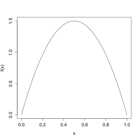
We'll take our discretization / bin width to be \(\Delta = 2^{-n}\), so we'll first divide up the interval into halves, then fourths, then eighths, etc. Since we know \(f(x)\), for each of these intervals we can apply the Mean Value Theorem to find the appropriate representative \(x_{i}\) in each \(I_{i}\). For example, here we take \(n = 2\) and \(\Delta = 1/2\):
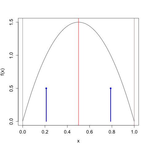
The red lines indicate the demarcations of the partitions, and the blue 'lollipops' indicate the mass assigned each \(x_{i}\). As expected, we choose two candidate points that put half the mass to the left of \(x = 1/2\) and half the mass to the right. All points to the left of \(x = 1/2\) get mapped to \(x_{0} = \frac{1}{2} - \frac{\sqrt{3}}{2} \approx 0.211\), all points to the right of \(x = 1/2\) get mapped to \(x_{1} = \frac{1}{2} + \frac{\sqrt{3}}{2} \approx 0.789\).
We can continue in this way, taking \(n\) larger and larger, and we get the following sequence of discretizations:
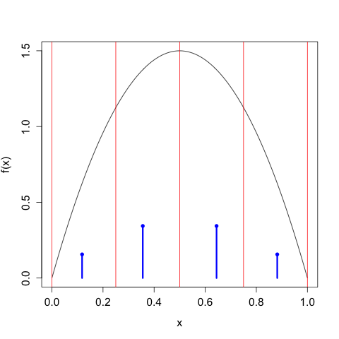
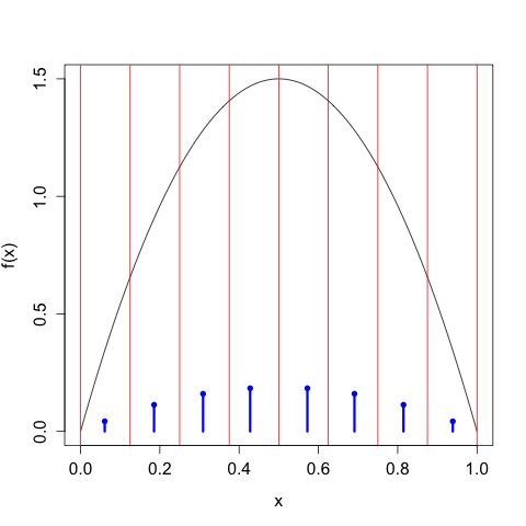
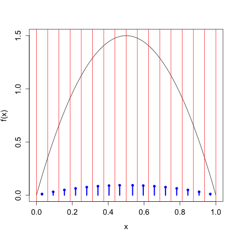
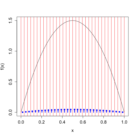
As we take our discretization to be finer and finer, the discrete entropy of \(X^{\Delta(n)}\) increases without bound, \[\begin{align} H\left[X^{\Delta(1)}\right] &= 1 \\ H\left[X^{\Delta(2)}\right] &= 1.896 \\ H\left[X^{\Delta(3)}\right] &= 2.846 \\ H\left[X^{\Delta(4)}\right] &= 3.828 \\ \vdots \\ H\left[X^{\Delta(4)}\right] &= 9.189, \end{align}\] We need to control this growth by tacking on the \(\log_{2} \Delta(n)\) term, in which case we have \[\begin{align} H\left[X^{\Delta(1)}\right] + \log_{2}(\Delta(1)) &= -1.110 \times 10^{-16} \\ H\left[X^{\Delta(2)}\right] + \log_{2}(\Delta(2)) &= -0.1039 \\ H\left[X^{\Delta(3)}\right] + \log_{2}(\Delta(3))&= -0.154 \\ H\left[X^{\Delta(4)}\right] + \log_{2}(\Delta(4))&= -0.172 \\ \vdots \\ H\left[X^{\Delta(10)}\right] + \log_{2}(\Delta(10))&= -0.1804, \end{align}\] which of course gets closer and closer to the differential entropy \(h[X] \approx -0.180470.\)
As usual, dealing with the continuum makes our lives a bit more complicated. We gain new machinery, but at the cost of our intuition.
In particular, because we have assumed that \(X\) admits a density, we know that \(f\) must be continuous, because otherwise it would not admit a density. For example, if it did have discontinuities, then probability mass would leave at those discrete points, and the density would not exist.↩