Excel Statistics

Attention Conservation Notice: Far too many words (again) on why I think (good) statistics matters and (bad) statistics should be destroyed.

I pontificate a lot about statistics. I knew it had gotten bad when a friend commented to me recently that he liked my rant, and I had to ask which one. I think I fight so hard for statistics because there was a period in my life (mostly my undergraduate years) when I thought statistics wasn't a field worth studying. It's just means, medians, and modes. We learned that stuff in elementary school. Why would anyone want to become a statistician?

After beginning to study nonlinear dynamics and complex systems, I saw statistics everywhere. A lot of it was shoddily done. Some of it was not. And then I took mathematical statistics the Spring semester of my senior year, and realized that statistics is not, in fact, a castle built in the sky. Rather, it's a castle solidly constructed, with foundations in measure theory. Lots of smart people worked on making it the field it is today. There are some philosophical differences amongst its practitioners, but overall the field offers a lot of tools for studying the stochastic world we live in.

And yet. And yet I still find myself frequently railing against statistics. Like when I see a course like this. Do I think that sociologists should learn more statistics? Yes. But not like this. No joke, one of the examples from the first day handout proposes doing a \(t\)-test to determine whether married or unmarried individuals have more sex.

And I quote:

People who are married have sex an average of 78 times a year; unmarried people have sex on average 53 times a year. The \(t\)-test value is 7.29 indicating that the difference is statistically significant.

The hypothesis is supported-cannot be rejected-given these measurements.

Let's not worry about whether the estimator they're using is asymptotically \(t\)-distributed. (Do these students even remember what asymptote means?) Much more important is that this question isn't interesting. Statistics got its start answering sociological questions, about life and death, crime and punishment. Poisson proved a generalization of the law of large numbers so that he could use it in designing a fair jury system for courts.

And now sociologists in training run \(t\)-tests to see who has more sex.

During an office conversation with a friend, we coined a new phrase: 'Excel statistics.' That's the sort of statistics this handout advocates. 'Let's do a hypothesis test, because that involves math! Which makes it science!'1 No. 'Let's a fit a line through the data, and report an \(R^{2}\) value!' No. 'Let's...'

Readily available computing has brought statistics to the masses. Which should be a good thing. Unfortunately, the masses aren't ready for statistics.

Maximum Likelihood and Entropy

Cosma Shalizi posted recently about optimization for learning. This is a recurring theme in statistics1: set up a functional combining empirical risk and a regularization term for smoothing, then use optimization to find a parameter value that minimizes this functional. Standard examples include ridge regression, LASSO, smoothing splines, support vector machines, and many, many more. As usual, Shalizi does a masterful job of introducing the key ideas behind this approach, even presenting a simple maximum likelihood example (for the Pareto distribution), along with R code.

After reading through his post and working through the Pareto distribution example, I realized two things: (i) I'd never really understood why maximum likelihood estimation works and (ii) I'd never really realized the important connection between log likelihoods and information theoretic quantities like entropy and Kullback-Leibler divergence. The first part is understandable: I've had this experience many, many times. The second part is embarrassing: both involve logarithms of mass / density functions, so the connection should have been obvious.

But even after making the second realization (the presence of logs in both subjects), I couldn't find any material explicitly making this connection. The closest thing from the cursory googling was this. But it didn't quite answer my question.

So, along the lines of my other post on entropy, let's follow the connection between maximum likelihood estimation and information theory to its completion. Consider this as a supplement to Shalizi's post, focusing explicitly on maximum likelihood estimation.

First, what is maximum likelihood estimation? Let's consider a random sample \(X_{1}, \ldots, X_{n}\) of random variables, all with common density2 \(f(x; \theta_{0})\). By specifying \(\theta_{0}\) like this, I'm assuming we're doing parametric inference: fixing a (possibly vector) parameter \(\theta_{0}\) and the probability family (like normal, exponential, Pareto, etc.) gives us the density \(f(x; \theta_{0})\) with which we can make any probability statement of interest. Of course, since we're doing statistical inference, \(\theta_{0}\) is unknown. Our goal is to figure it out: we formulate a good statistic of the data \(X_{1}, \ldots, X_{n}\), call it \(T\), and estimate our parameter as \(\hat{\theta} = T(X_{1}, X_{2}, \ldots, X_{n})\). A statistic that you're familiar with is the sample mean of a random sample,

\[T(X_{1}, \ldots, X_{n}) = \frac{1}{n} \sum_{i = 1}^{n} X_{i}.\]

The maximum likelihood method for determining \(\hat{\theta}\) is as follows. Write down the joint density of the random sample, \[\begin{align*} f_{X_{1}, \ldots, X_{n}}(x_{1}, \ldots, x_{n}; \theta) &= f_{X_{1}}(x_{1}; \theta) \ldots f_{X_{n}}(x_{n}; \theta)\\ &= \prod_{i = 1}^{n} f_{X_{i}}(x_{i}; \theta) \\ &= \prod_{i = 1}^{n} f_{X}(x_{i}; \theta) \end{align*}\] where the factorization of the joint density comes from independence and the last line follows from the identical-ness of the sample. Notice that we're not fixing \(\theta\). Remember: we don't know \(\theta\). So we can think of this joint density as a function of \(\theta\), as well as a function of the arguments \((x_{1}, \ldots, x_{n}).\) When we think of the density from this perspective, we call it the likelihood, and would usually write \[L(\theta; x_{1}^{n}) = \prod_{i = 1}^{n} f_{X}(x_{i}; \theta)\] where \(x_{1}^{n}\) is shorthand for the vector \((x_{1}, \ldots, x_{n})\). We then evaluate the likelihood at our random sample, which gives us \[L(\theta; X_{1}^{n})\] and choose the \(\theta\) value that maximizes. That is, we take our estimator to be \[ \hat{\theta} = \arg \max_{\theta} L(\theta; X_{1}^{n}).\] Of course, \(X_{1}^{n}\) is random, and thus \(L(\theta; X_{1}^{n})\) is a random function, making \(\hat{\theta}\) a random variable. Sometime we can find an explicit function mapping us from the sample to the statistic, in which case we could write \(\hat{\theta} = T(X_{1}, X_{2}, \ldots, X_{n}).\) If not, we proceed by numerical optimization.

In words, we choose the parameter value that maximizes the likelihood of the data. This makes intuitive sense, but why does it work?

In practice, we minimize the negative log-likelihood. That is, we seek \[ \hat{\theta} = \arg \min_{\theta} - \log L(\theta; X_{1}^{n}).\] All the times I've seen this presented, the usual reason given is that this approach turns products into sums, which makes the minimization easier. This is true, but there's a deeper reason for doing this. The logarithm puts us into the domain of information theory, which we can use to show that maximum likelihood makes sense3.

Let's pull the logarithm through the product, giving \[- \log L(\theta; X_{1}^{n}) = - \sum_{i = 1}^{n} \log f(X_{i}; \theta).\] Finally, if we divide by \(n\), giving us the sample negative log-likelihood, we get \[- \frac{1}{n} \sum_{i = 1}^{n} \log f(X_{i}; \theta).\] I got stuck here for a while. By the (Strong or Weak) Law of Large Numbers, this should converge to its expected value (almost surely or in quadratic mean). More specifically, by the asymptotic equipartition theorem, I thought this should converge to the differential entropy of \(X\), namely \[h[f(x; \theta_{0})] = - E[\log f(X; \theta_{0})] = - \int_{\mathbb{R}} f_{X}(x; \theta_{0}) \log f_{X}(x; \theta_{0}) \, dx\] But we have to be careful about how we take the expectation. We have \[- \frac{1}{n} \sum_{i = 1}^{n} \log f(X_{i}; \theta).\] which doesn't fix \(\theta\) at \(\theta_{0}\), and the asymptotic equipartition theorem tells us \[- \frac{1}{n} \sum_{i = 1}^{n} \log f(X_{i}; \theta_{0}) \to h[f(x; \theta_{0})],\] but nothing about how \[- \frac{1}{n} \sum_{i = 1}^{n} \log f(X_{i}; \theta)\] should behave. To get to where we're going, we have to pull the usual mathematical trick of adding zero. If we pull the negative inside and then add and subtract the log-likelihood under the true model, we get \[\begin{align} \frac{1}{n} \sum_{i = 1}^{n} \left\{- \log f(X_{i}; \theta) + \log f(X_{i}; \theta_{0}) - \log f(X_{i}; \theta_{0})\right\} &= \frac{1}{n}\sum_{i = 1}^{n} \left\{ \log \frac{f(X_{i}; \theta_{0})}{f(X_{i}; \theta)} - \log f(X_{i}; \theta_{0}) \right \} \\ &= \frac{1}{n}\sum_{i = 1}^{n} \log \frac{f(X_{i}; \theta_{0})}{f(X_{i}; \theta)} - \frac{1}{n}\sum_{i = 1}^{n} \log f(X_{i}; \theta_{0}) \end{align}\] Now this converges (again, either almost surely or in quadratic mean) to \[ D_{KL}(f(x; \theta_{0}) || f(x; \theta)) + h[f(x; \theta_{0})],\] where \[ D_{KL}(f(x; \theta_{0}) || f(x; \theta)) = \int_{\mathbb{R}} f(x; \theta_{0}) \log \frac{f(x; \theta_{0})}{f(x; \theta)} \, dx\] is the Kullback-Leibler divergence or relative entropy between \(f(x; \theta_{0})\) and \(f(x; \theta)\). Thus, we see that the mean negative log-likelihood converges to the differential entropy under the true distribution plus the Kullback-Leibler divergence between the true distribution and the distribution we guess at. One can show4 that the Kullback-Leibler divergence is non-negative and is zero only when \(f(x; \theta_{0}) = f(x; \theta)\) almost surely. Recalling that we're seeking to minimize the mean negative log-likelihood, this means that we want to choose \(\theta = \theta_{0}\) to minimize this limiting function.

And after a bit of a detour through information theory, we've seen a sketch as to why Maximum Likelihood Estimation makes sense as a procedure for estimating a parameter \(\theta\). The mean negative log-likelihood converges to a non-random function, and that non-random function takes its minimum at the correct answer to our question. Fully proving consistency of the maximum likelihood estimator requires a good deal more work.

But that's the beauty of sketches.


  1. And machine learning. But a lot of people always overlook statistics when talking about learning, so I'll show my prejudice.

  2. I'm technically going to be talking about differential entropy throughout, since the Pareto distribution from Shalizi is a continuous distribution. But the same results hold for discrete distributions and thus discrete (aka Shannon) entropy.

  3. I'm going to be super hand-wavy here. Less hand-wavy than an undergraduate statistics class, for sure, but too hand-wavy for a graduate asymptotic statistics class. My apologies.

  4. And I won't. The proof involves an application of Jensen's inequality.

Lines, Springs, and Statistical Thinking

Attention Conservation Notice: A lesson that you can use any statistical method you want, but some are certainly better than others.

I follow Rhet Allain's blog Dot Physics. In fact, his most recent post about replacing the terms 'hypothesis', 'theory', and 'scientific law' with 'model' in the scientific lexicon is spot on. That's something I feel extremely comfortable with as a mathematician: 'most models are wrong, some are useful.'

But another recent post of his, about finding the spring constant for a spring-mass system made my ears perk up. In high school and college, my favorite part of labs was always the data analysis (and my least favorite part was the labwork, which goes a long way towards explaining why I'm now training to be a mathematician / statistician).

With the briefest of introductions, the model for a spring-mass system (without drag) falls out of the linear, second-order, constant coefficient ordinary differential equation1

\[m y'' + ky = 0\]

where \(y\) is the displacement of the spring away from its equilibrium position, \(m\) is the mass on the spring, and \(k\) is the spring constant. This follows directly from Hooke's law2, namely that the force acting on the mass is proportional to the negative of the displacement away from the equilibrium position, with the proportionality tied up in this thing we call the spring constant \(k\). From this alone we can derive the equation that we're interested in, namely the relationship between the period of a spring's oscillation and the spring constant. Skipping over those details, we get that

\[T = \frac{2 \pi}{\sqrt{k}} \sqrt{m}.\]

The usual lab that any self-respecting student of the sciences has performed is to place various different masses on the spring, displace the mass a bit from its equilibrium position, and measure its period (hopefully over a few cycles). Once you have a few values \((m_{1}, T_{1}), \ldots, (m_{n}, T_{n})\), you can then go about trying to find the spring constant. Doing so is of course a matter of regression, which brings us into wheelhouse of statistics.

And since we're in statistics land, let's write down a more realistic model. In particular. the thing that is being measured (and by undergraduates, even!) is the period as a function of the mass. Undergraduates are a fickle lot, with better things to think about then verifying a 350+ year old law. Their attention may waver. Their reaction speed may be lacking. Not to mention physical variations in the measurement system. All of this to say that the model we really3 have is

\[T_{i} = \frac{2 \pi}{\sqrt{k}} \sqrt{m_{i}} + \epsilon_{i}\]

where \(\epsilon_{i}\) is an additive error which, for the sake of simplicity, we'll assume has mean zero and variance \(\sigma^{2}\) not depending on \(m\). We'll also assume the errors are uncorrelated. This isn't so unreasonable of a model, compared to some of the probabilistic models out there.

As written, it seems obvious what we should do4. Namely, the model for \(T\) is linear in \(\sqrt{m}\), and we know the values of the \(m_{i}\) (to pretty high precision, if I recall correctly from my college physics days). On top of that, the Gauss-Markov theorem tells us linear regression is the best we can do to find the spring constant (out of the class of all unbiased estimators for it). So we should fit a linear regression of \(T\) against \(\sqrt{m}\), and read off \(k\) by simple algebra.

Allain takes a different tact, which at first seems just as good. Namely, he notices that if we square both sides of

\[T = \frac{2 \pi}{\sqrt{k}} \sqrt{m},\]

we get

\[T^{2} = \frac{(2 \pi)^{2}}{k} m,\]

which is now linear in \(T^{2}\) and \(m\). We can fit a line through the points \((m_{i}, T_{i}^{2})\) just as we would have with my method, and read off \(k\) in a similar fashion. But the problem with this approach is that the model isn't right. Remember, the actual model has error in it,

\[T_{i} = \frac{2 \pi}{\sqrt{k}} \sqrt{m_{i}} + \epsilon_{i},\]

so when we square the period, we get

\[T_{i}^{2} = \frac{(2 \pi)^2}{k} m_{i} + 2 \frac{2 \pi}{\sqrt{k}} \sqrt{m_{i}} \epsilon_{i} + \epsilon^{2}_{i}.\]

This is much uglier. And adds a bias to our model. In particular, note that

\[E[T_{i}^{2}] = \frac{(2 \pi)^2}{k} m_{i} + E[\epsilon^{2}_{i}] = \frac{(2 \pi)^2}{k} m_{i} + \sigma^{2}.\]

So as we add more measurement noise, we'll get more and more biased from the true value of the spring constant5.

This is a lot of math to say what every experimentalist already knows: when dealing with propagation of errors, it's best to manipulate the thing that has the least amount of error in it. In this case, that means taking the square root of the mass instead of squaring the period.

Theory is nice, but let's follow Allain's lead and do some simulations. I'll take the true value of the spring constant to be \(k = 13.5\), as Allain does in his post. I simulate from the model

\[T_{i} = \frac{2 \pi}{\sqrt{k}} \sqrt{m_{i}} + \epsilon_{i},\]

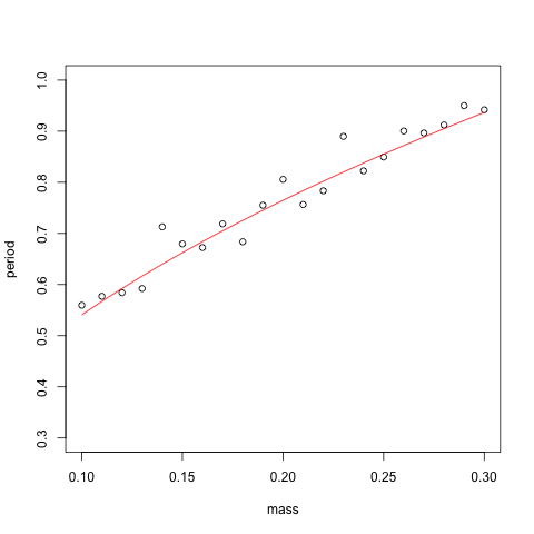
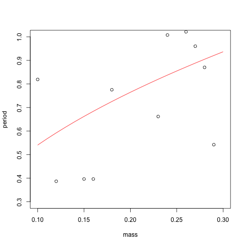
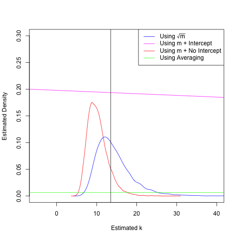
for each value of \(m_{i}\), and do this \(B = 10000\) times6,7. I took \(\epsilon_{i} \sim N(0, \sigma^{2})\), with various different values for \(\sigma\). Allain initially took his \(\epsilon_{i}\) to be Uniform(-1/20, 1/20), so I used that to get an equivalent variance for the normal case, namely \(\sigma = \sqrt{1200} \approx 0.03\). Below I've plotted both what the noisy data looks like (with the true regression curve in red), and the distribution of our different estimators over the 10000 trials.

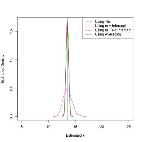
In the presence of low noise, all but the method that estimates both an intercept and a slope do about equally well8. This is good to know. But we would like our methods to continue to work well in the case of large amounts of noise. I can't stress this enough: these experiments are being performed by undergraduates!

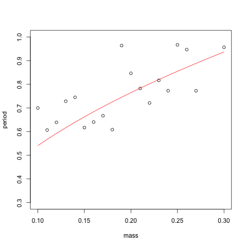
So, let's bump up the noise to \(\sigma = 0.1\). This means that 95% of the time, the noise will only push us away from the true period by a magnitude of 0.2 seconds. That's doesn't seem like an unreasonable amount of uncertainty to allow in our period recording procedure. And here's the result:

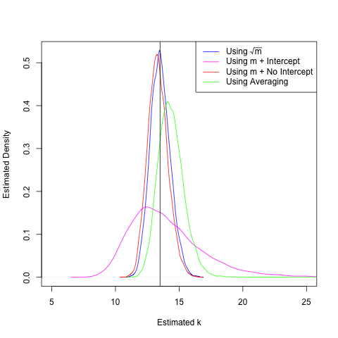
We can already see the bias creeping into our \(T^2\)-based estimators. Only the regression method using \(\sqrt{m}\) gives a density sharply peaked around the true value. This is unsurprising, given our analysis above, but also comforting. Finally, let's take the noise to an even greater extreme and use \(\sigma = 0.5\). This means that 95% of the time, we'll be off by at most a second from the true value of the period. This is an unreasonable amount of noise (unless the undergraduate performing the lab has had a particularly bad day), but it demonstrates the strengths and weaknesses of the various estimators for \(k\).

At this point, the densities need no explanation. Of the methods proposed in Allain's post, only the '\(m +\) No Intercept' method stills stays in the right ballpark of the true value of \(k\), but is biased by the squaring procedure. I can't stress enough that this amount of noise is unreasonable, especially since the students are presumably measuring the period over several oscillations and thus have the Law of Large Numbers on their side. But it does demonstrate the importance of thinking carefully (and statistically!) about how we would like to do our data analysis.

I have fond memories from my undergraduate days of manipulating equations until they were linear in the appropriate variables, and then fitting a line through them to extract some sort of physical quantity. At the time of that training, I had no statistical sophistication whatsoever. Understandably so. There's barely enough time to cover the science in standard science courses. But it would be nice (for both theorists- and experimentalists-in-training) if a little more statistical thinking made it into the curriculum.

For the sake of reproducibility, I have made my R code available here.


  1. Can you tell I've TAed Elementary Differential Equations twice at UMD?

  2. To have lived when you could have such a simple law named after you!

  3. Not in the ontological sense, but rather in the sense of being more useful.

  4. Though 'obvious' is a loaded word. I've been spending too much time thinking about regression, in all its various forms, lately.

  5. Unless we add an (artificial) intercept to our regression model. The nice thing about (simple) physical models: we have reasons to include / not include parameters in our regression.

  6. Simulation is a wonderful thing. And we've come a long way since when statisticians had to flip coins to get statistical fodder. I read a story once about Eugen Slutsky's study of apparent cycles in economic data. In the process of performing his simulations, he really did flip a coin thousands of times to simulate a random walk. Unfortunately, I can't find the article where I originally read this, so I'll just state it as a anecdote and hope I'm not misremembering.

  7. You'll also notice that I took my masses (called 'design points' in the jargon of regression) to be at more regularly spaced intervals. Namely, I took them to be from 0.2 to 0.3, with spacing 0.01. This seems like a reasonable enough choice of masses, though again, asking our undergraduate to measure 21 periods may be a bit much. Besides, we certainly won't do better with less design points than this.

  8. The degradation in performance for the '\(m +\) Intercept' model can be explained in terms of the well-known bias-variance tradeoff. But adding the intercept term to our squared period model, we've allowed the slope to be estimated correctly (by capturing the \(\sigma^{2}\) term within the intercept), thus reducing the bias. But by forcing our procedure to estimate two quantities, we've increased the variance in both. In other words: if physics tells us to use a simpler model, for heaven's sake, use the simpler model!

Good Statistics

When it comes to meta-models of statistics, here are two philosophies that I respect:

  1. (My) Bayesian approach, which I associate with E. T. Jaynes, in which you construct models with strong assumptions, ride your models hard, check their fit to data, and then scrap them and improve them as necessary.
  1. At the other extreme, model-free statistical procedures that are designed to work well under very weak assumptions-for example, instead of assuming a distribution is Gaussian, you would just want the procedure to work well under some conditions on the smoothness of the second derivative of the log density function.

Both the above philosophies recognize that (almost) all important assumptions will be wrong, and they resolve this concern via aggressive model checking or via robustness. And of course there are intermediate positions, such as working with Bayesian models that have been shown to be robust, and then still checking them. Or, to flip it around, using robust methods and checking their implicit assumptions.

See. Frequentists can do good statistics, too.

If it's not obvious, I prefer the second approach.

Why Entropy?

There are many ways to define the entropy of a random variable. Claude Shannon originally justified his choice on axiomatic grounds. If we force our functional \(H[p(x)]\) to satisfy three properties, then the form of entropy as

\[H[p(x)] = - E[log_{2}(p(X))]\]

falls out of the requirements on \(H[p(x)]\).

A less formal, but equivalent, definition of entropy is in terms of the minimum expected number of binary questions needed to identify the value of a discrete random variable \(X\). This is (from personal experience) a typical starting point for introducing entropy. Let's take this approach, but then follow it to completion1.

We'll start with the example from Cover and Thomas. Let \(X\) be a discrete random variable taking values from the 'alphabet'2 \(\mathcal{X} = \{ a, b, c, d\}\). Thus, we can specify \(X\) by giving its probability mass function,

\[p(x) = P(X = x) = \left\{ \begin{array}{cc} \frac{1}{2} &: x = a \\ \frac{1}{4} &: x = b \\ \frac{1}{8} &: x = c \\ \frac{1}{8} &: x = d \end{array}\right. .\]

Our goal is to ask a series of binary questions of the form 'Is \(X =\) ?' and get the answer 'Yes!' as quickly as possible. Of course, \(X\) is a random variable, so the number of questions we will have to ask isn't a number, but a random variable itself. Thus, we can formalize our goal as follows: we want to minimize the expected number of questions we'll have to ask to get at the identity of \(X\). Call this quantity \(\bar{\ell}\) (the reason for this choice will become clear later on). We can work out this value for the probability mass function above. But first, we have to specify the procedure that we'll use to ask the questions. The obvious choice, and the one we'll make, is to ask first if \(X = a\)? (since \(a\) is the most probable value), and then \(b\), and then \(c\), and so on, until we've arrived at the correct value for \(X\). Given this strategy, we'll ask a single question \(1/2\) of the time (since \(P(X = a) = 1/2\)), two questions 1/4 of the time, and 3 questions 1/8 + 1/8 = 1/4 of the time3. Thus, the expected number of questions we'll have to ask is

\[ \bar{\ell} = \frac{1}{2} \cdot 1 + \frac{1}{4} \cdot 2 + \frac{1}{8} \cdot 3 + \frac{1}{8} \cdot 3 = 1.75.\]

A quick computation shows that 1.75 is also the entropy of \(X\), since4

\[ \begin{align} H[X] &= -\sum_{x \in \mathcal{X}} p(x) \log p(x) \\ &= -\left(\frac{1}{2} \cdot \log \frac{1}{2} + \frac{1}{4} \cdot \log \frac{1}{4} + \frac{1}{8} \cdot \log \frac{1}{8} + \frac{1}{8} \cdot \log \frac{1}{8}\right) \\ &= 1.75. \end{align}\]

Thus, for this case, the entropy and the minimum number of expected questions turn out to coincide. This only occurs when \(p(x)\) is a dyadic distribution5. In the general case where \(p(x)\) is not dyadic, the minimum expected number of questions is bounded between entropy and entropy plus 1. That is, in general,

\[ H[X] \leq \bar{\ell}^{*} < H[X] + 1.\]

Why this should be the case will (hopefully) become more clear in a moment.

Okay, so far we haven't done anything beyond the standard approach taken in Cover and Thomas. But now let's formalize our question asking process a little, and see how we can relate it to data compression. The goal of lossless data compression is to map an alphabet \(\mathcal{X}\) into a new alphabet \(\mathcal{D}\) (which we'll take to be binary, namely \(\mathcal{D} = \{ 0, 1\}\)) as to make the encoded words as short as possible, in expectation. There are a lot of results from data compression. The main result we'll need is the optimality of Huffman codes. I won't go into the details of what a Huffman code is, but suffice it to say this code will get us the question procedure that gives us the minimum expected number of binary questions.

Here is how we will use the Huffman code to encode our alphabet \(\mathcal{X} = \{a, b, c, d\}\). We'll map each element of \(\mathcal{X}\) into a binary string which keeps track of the number of questions we asked as well as the answers to those questions. We'll use the same questioning procedure as before, which will give us the mapping

\[\begin{align} a &\to 1 \\ b &\to 01 \\ c &\to 001 \\ d &\to 000. \end{align}\]

Again, we'll read each binary string from left to right. Thus, the string that \(a\) maps to, namely 1, says, "We've asked 'Is \(X = a\)?' and gotten the answer 'Yes.'" The string that \(b\) maps to says, "We've asked 'Is \(X = a\)?' and gotten the answer 'No.' We then asked 'Is \(X = b\)?' and gotten the answer 'Yes.'" To go one further, the string that \(d\) maps to says, "We've asked 'Is \(X = a\)?' and gotten the answer 'No.' We then asked 'Is \(X = b\)?' and gotten the answer 'No.' We then asked 'Is \(X = c\)?' and gotten the answer 'No.'" (Thus, \(X = d\), by exhaustion of the possibilities.) Note that this code is not unique (for example, we could have asked about \(d\) before asking about \(c\), or interchanged the roles of 0 and 1), but it is optimal.

So now we have a way to formulate our question procedure in an optimal way, and we see that the length of each codeword corresponds to the number of questions we had to ask to get at \(X\)'s identity. Therefore, the expected length of a codeword is equal to the expected number of binary questions, and we have made the missing link between data compression and binary questions.

We still haven't shown that the optimal questioning strategy results in an expected number of binary questions between entropy and entropy plus 1. To get this result, we can now turn again to the ample literature on coding theory, and realize that the Huffman code, which we used to construct our procedure, is a prefix code. One of the (many) nice things about prefix codes is that they satisfy Kraft's inequality. Namely, if for each \(x_{i} \in \mathcal{X}\) we specify a code length \(\ell_{i}\), which is the number of digits that \(x_{i}\) maps to6, and the code is a prefix code, then Kraft's inequality requires that

\[ \sum_{i = 1}^{|\mathcal{X}|} D^{-\ell_{i}} \leq 1,\]

where we have assumed a \(D\)-ary encoding. (For a binary encoding, we took \(D = 2\).) This restriction, by itself, allows us to demonstrate that the expected code length (which, remember, is in a one-to-one mapping with the expected number of binary questions) must be greater than entropy7. To show that the expected code length of the optimal code is bounded above by entropy plus 1, we construct a simpler, but sub-optimal code, called the Shannon-Fano code, which it is easy to show is bounded above by entropy plus 1. Since our Huffman code is optimal, and thus better than the Shannon-Fano code, we must get that overall

\[ H[X] \leq \bar{\ell}^{*} < H[X] + 1\]

where \(\bar{\ell}^{*}\) is the expected code length (expected number of binary questions) for the optimal code ( optimal question procedure).


  1. Following the idea to its natural, and final, conclusion is not something that seems typical. In Cover and Thomas's Elements of Information Theory, for example, the definition of entropy in terms of the minimum expected number of binary questions is given, but then not justified beyond a single example. They promise a justification in Chapter 5 of the text, which covers Data Compression. But as far as I can tell (and I haven't made a careful reading of that chapter), they do not then make the key connection between data compression and entropy that they allude to in Chapter 1. Admittedly, the connection is obvious (if you think about it long enough), but I still the it's worth stating explicitly. A quick Google search found no mentions of this explicit connection, so maybe this post can fill that void.

  2. Information theory is overflowing with these electrical engineering-specific words: alphabet, code word, etc. As someone coming to the topic from a probabilistic / statistical background, this can be off-putting at times. But I have to remind myself that the electrical engineers made the first go at information theory, so they have earned the right to name things as they please.

  3. Note that we only ever have to ask at most 3 questions. With \(n\) possible values, we'll always have to ask at most \(n - 1\) questions, since on the last question, we know the identify of \(X\) even if the answer is no (we don't need an \(n^\text{th}\) question to identify \(X\)).

  4. From here on out, all logarithms are taken base 2.

  5. Or to be more exact, when the distribution is \(D\)-adic, where we take our encoded alphabet to be \(\mathcal{D} = \{ 0, 1, \ldots, D- 1\}\). The dyadic case is a special case where \(D = 2.\)

  6. In the previous example, the length of the codeword \(a\) maps to is \(1\), so \(\ell_{a} = 1\). Similarly, \(\ell_{b} = 2, \ell_{c} = 3\), and \(\ell_{d} = 3\).

  7. The proof is slick, and only involves a straightforward normalization and a simple tool from Information Theory. Of course, as with all slick proofs, it requires a trick that only seems obvious after the fact.

Mind the Gap

Larry Wasserman recently had a post about the gap between the development of a statistical method, and the justification of that method. He gives timelines for various methods, from the standard (like Maximum Likelihood Estimation) to the now-becoming-standard (like Causal Inference), demonstrating the large amount of time that had to pass between when inventors propose a method and when researchers (sometimes the same as the inventors!) prove results about why that method 'makes sense.'

I suppose, for the non-mathematically inclined reader, that I have to explain a little what I mean by 'makes sense.' Any method can be proposed to solve a problem (statistical or otherwise). But for statistical problems, we (sometimes) have the tools to answer whether or not we'll get the right answer, most of the time, with a given method.

As an illustrative example, consider the goal of determining the exponent of a power law model for the distribution of some empirical phenomena. This is a favorite topic of a lot of complex system scientists, especially physicists. For those with no training in statistics (beyond what they get in their undergraduate lab courses), a logical approach might be computing the empirical distribution function of the data, taking the logarithm of that function, and fitting a line through it1. If the data are power law distributed, then the true2 cumulative distribution function of the data will be a power law, and thus the log cumulative distribution function will be linear. Taking the slope of the line of best fit would give an affine transformation of the exponent, and our job is done.

Except that we don't have the true cumulative distribution function. Instead, we have the empirical distribution function, which is itself a stochastic process with some underlying distribution. In the limit of infinite data, the empirical distribution will converge to the true distribution function almost surely. But in the meantime, we don't have many guarantees about it, and we certainly don't know that it will give us a good estimate of the exponent of the power law.

Instead, we should use Maximum Likelihood Estimation, as proposed by Ronald Fisher (and perhaps first used by Carl Friedrich Gauss in some computations about celestial orbits). This method is standard statistical fair3, and its application to power laws is well documented. And unlike the line-of-best-fit-through-the-empirical-distribution-function method, it has provably nice properties. And yet people still continue to use the line-of-best-fit method. Why? Because it makes intuitive sense. But it doesn't 'make sense,' statistically.

All of that to explain the (research) nightmares that keep me up at night: using (or worse, proposing!) a method that doesn't 'make sense.' Which is why Larry Wasserman's post is so consoling. Perhaps I don't immediately know why a method I would like to use makes sense. But hopefully in the future, someone far smarter than me will derive the justification for my method.

To quote Cosma Shalizi, from Section 11.4.3 of his thesis, where he proposes using computational mechanics for continuous-valued, discrete-time stochastic process,

It becomes a problem of functional analysis, so the mathematical foundations, if we aim at keeping to even the present standard of rigor, will get much more complicated. Still, we might invoke the physicist's license to ignore foundations, on the grounds that if it works, the mathematicians will find a way of making it right.

For those interested, he has since made this leap. See his and his graduate student Georg Georg's work on LICORS.

Wasserman's post was prescient. Rob Tibshirani, one of the co-inventors of the LASSO (an \(\ell_{1}\)-regularized least squares method), recently developed a significance test for the LASSO (one of the methods listed in Wasserman's 'The Gap' post). This provides even more (statistically justified!) tools for using the LASSO.

Which means that the method now 'makes sense' even more.


  1. Admittedly, this is the favorite approach of a lot of people, not just physicists. But for a group supposedly interested in nonlinear science, the use of a linear method seems suspect.

  2. Okay, 'true' here may be a bit too strong of a word. Let's say 'a good model of the data generating process.'

  3. I learned about it in my undergraduate mathematical statistics course.

Silver at the Oscars

As part of the Directed Reading Program I'm doing with a student at Maryland, we've decided to dig into Nate Silver's Oscar Predictions for this year.

'Fortunately' for us, Silver only gives us a glimpse of his methodology. He also doesn't supply us with the data he used. I've compiled that data here. In short, here is his approach:

The gory details: I weight each award based on the square of its historical success rate, and then double the score for awards whose voting memberships overlap significantly with the Academy.

I don't know how a weighted average counts as 'gory,' but I guess Silver has a different audience in mind. Let's unpack this methodology, in the hopes that "by relieving the brain of all unnecessary work, a good notation sets it free to concentrate on more advanced problems."1

Let \(O^{(j)}\) be the Oscar winner in the \(j^{\text{th}}\) year, \(j = 1, \ldots, 25\). Let \(C_{i}^{(j)}\) be the award winner from the \(i^{\text{th}}\) ceremony, \(i = 1, \ldots, 16\)2. Let \(S^{(j)}\) be the set of candidate Oscar winners on the \(j^{\text{th}}\) year. For example, this year we had \[S^{(26)} = \{\text{Amour, Argo, Beasts of the Southern Wild, Django Unchained,}\]

\[\text{Les Miserables, Life of Pi, Lincoln, Silver Linings Playbook, Zero Dark Thirty} \}.\] Thus, we have nine films to predict from, and \(|S^{(26)}| = 9.\) From the description above, Silver wants to construct a function from \(S^{(26)}\) to the reals such that

\[ f(s) = \sum_{i = 1}^{16} \beta_{i} I[C_{i}^{(26)} = s], s \in S^{(26)}.\]

Here \(I[\cdot]\) is the indicator function, which is 1 if its argument is true, and 0 otherwise. For example, if \(s\) = Argo and \(C_{1}^{(26)} =\) Argo, then \(I[C_{1}^{(26)} = s] = 1.\) But if \(s\) = Argo and \(C_{2}^{(26)} =\) Amour, then \(I[C_{2}^{(26)} = s] = 0\). We then choose the film \(s\) that gets the highest weighted vote,

\[ \hat{s} = \arg \max_{s \in S^{(26)}} f(s).\]

Let's consider a few choices of \(\beta_{i}\) and see what sort of prediction they give us. If we take \(\beta_{i} = 1\) for all \(i\), our predictor reduces to

\[f(s) = \sum_{i = 1}^{16} I[C_{i}^{(26)} = s], s \in S^{(26)},\]

which, after arg max-ing, is simply the majority vote. That is, we'll choose the film that got the most awards from the non-Oscar awards that year. This seems like a reasonable enough predictor in the situation where we have no other information about how the the non-Oscar awards relate to the Oscar awarded on a given year. But we do have such information. It's summarized in Nate Silver's table and captured in this tab-delimited file. We can (hopefully) use the past performance of the non-Oscar awards and the Oscars to predict how the Oscars will turn out this year. Loosely, we can try to pick up on correlations between the non-Oscar awards and the Oscars that might be predictively useful. This is exactly what Silver ends up doing, in an ad hoc fashion.

Using the historical data, Silver computes, for each award \(i\), the fraction of years that award and the Oscars agreed on their winning films. Using our handy-dandy indicator functions again, we can write this value \(\hat{p}_{i}\) as

\[\hat{p}_{i} = \frac{1}{n_{i}} \sum_{j = 1}^{n_{i}} I[O^{(j)} = C_{i}^{(j)}]\]

where \(n_{i}\) is the number of years we have data for award ceremony \(i\), since not all of the award ceremonies go back to 1987. In fact, only ten of the fourteen I've included do. With the \(\hat{p}_{i}\) values in hand for all of the sixteen non-Oscar awards, Silver computes his new weighted vote3 as

\[ f(s) = \sum_{i = 1}^{16} \hat{p}_{i}^2 I[C_{i}^{(26)} = s], s \in S^{(26)}.\]

How does this compare to the 'majority vote' predictor above? Now we account for the number of votes given to each of the candidate films, and how those votes match up with Oscars in the past. In other words, if a lot of the non-Oscar awards vote for a film, but those awards also haven't matched the Oscars winner historically, we'll discount their votes.

So far we've seen two possible choices for the weights \(\beta_{i}\). The first choice for the weights, namely \(\beta_{i} = 1\) for all \(i\), work well in the situation where we have no historical information. The second choice, namely \(\beta_{i} = \hat{p}_{i}^{2}\) seems reasonable enough when all we know is whether a non-Oscar award agreed or didn't with the Oscars in the past. But why the square? And can we choose a different weighting that gets us more standard predictor from the statistical learning literature4?

Stay tuned to find out!


  1. A new favorite quote by Alfred Whitehead.

  2. Note that Nate Silver uses 16 awards instead of my 14. I removed the American Cinema Editors Award for Best Comedy or Musical and the Golden Globe for Best Musical or Comedy, since they didn't seem to have much to do with the Best Film, which is usually a Drama.

  3. Well, not quite yet. Silver also doubles the weight for 'insider' awards. These are awards that have a considerable overlap with the Oscars in terms of their members. So, add that doubling to the model to get back Silver's complete predictive model.

  4. My current gut feeling: this feels a lot like logistic regression. We're basically doing a multi-class classification problem. But the fact that the set of films changes every year complicates things a bit.

High School Chemistry — Accuracy and Precision

High school chemistry was the first time I heard the words 'accuracy' and 'precision' in a scientific context. The terms were presented by way of a bullseye example (more on that later), and the Wikipedia article on the topic captures the gist pretty well:

In the fields of science, engineering, industry, and statistics, the accuracy of a measurement system is the degree of closeness of measurements of a quantity to that quantity's actual (true) value. The precision of a measurement system, also called reproducibility or repeatability, is the degree to which repeated measurements under unchanged conditions show the same results. Although the two words reproducibility and repeatability can be synonymous in colloquial use, they are deliberately contrasted in the context of the scientific method.

See the Wikipedia article for the standard bullseye figures.

At the time (some nine years ago now), my friends and I would frequently get confused about which was which. Did precision relate to how close to the bullseye you were? Did accuracy relate to how closely grouped the points were? The names themselves didn't really clarify anything. Precise and accurate sound, to the teenage ear, indistinguishable.

While reading through Nate Silver's The Signal and the Noise, I had the (strikingly obvious) realization that these terms could easily be framed in probabilistic language1. I don't think 10th-grade-me would have understood this framing. But that's his fault, not mine.

Here's the setup. Suppose we have some true value, \(\theta\), that we would like to measure. Maybe it's the speed of light in a vacuum, or the volume of water in our volumetric flask. Call our measurement of that value on a single trial \(\mathbf{M}\), and take \(\mathbf{M}\) to be given by

\[\mathbf{M} = \theta + \mathbf{N}.\]

Here, \(\mathbf{N}\) is 'noise.' For example, it might be noise due to measurement apparatus. Basically, \(\mathbf{N}\) will capture all of the things that could go wrong in the process of making the experimental measurement.

Let's choose to model \(\mathbf{N}\) in a simple way. I do this because it makes operationalizing precision and accuracy much easier. We'll assume that

\[\mathbf{N} \sim \text{Normal}(\mathbf{b}, \Sigma)\]

(Hold for all of the comments about why Normal theory is the devil.)

Okay, so we're assuming that the errors in our measurement are normal with mean \(\mathbf{b}\) and covariance \(\Sigma\). And now we're done. The precision of our measurement \(\mathbf{M}\) has to do with how 'small' \(\Sigma\) is. So that I can use the bullseye example, \(\mathbf{M}\) is a vector in \(\mathbb{R}^{2}\), so \(\Sigma\) is a \(2 \times 2\) matrix of covariances

\[(\Sigma)_{ij} = \text{Cov}(N_{i}, N_{j}).\]

This shows us that precision is a relative term: you can always be more or less precise, depending on how small you can make \(\text{Var}(N_{1})\) and \(\text{Var}(N_{2})\).

Accuracy, on the other hand, has to do with \(\mathbf{b}\), the suggestively named bias of our measurement process. If \(\mathbf{N} \sim \text{Normal}(\mathbf{b}, \Sigma)\), then \(\mathbf{M} \sim \text{Normal}(\theta + \mathbf{b}, \Sigma)\). In other words, \(\mathbf{M}\) picks up the bias in our measurement apparatus. No amount of averaging of the measurements will get us the right value. Sorry Law of Large Numbers, we'll always be off from \(\theta\) (on average) by \(\mathbf{b}\). Thus, accuracy is absolute (according to our model): we're either accurate, or we're not.

Now some pictures to clarify this result. We stick with the bullseye example, because it really is nice. As the Wikipedia article states, we can be:

  • precise and accurate, which means that \(\Sigma\) is small and \(\mathbf{b} = \mathbf{0}\)
  • precise and not accurate, which means that \(\Sigma\) is small and \(\mathbf{b} \neq \mathbf{0}\)
  • not precise and accurate, which means that \(\Sigma\) is large and \(\mathbf{b} = \mathbf{0}\)
  • not precise and not accurate, which means that \(\Sigma\) is large and \(\mathbf{b} \neq \mathbf{0}\)

For some reason, the standard textbooks (i.e. the textbooks I learned high school chemistry from) focus on only a few of these cases. All four cases, in the order above, are presented below.

So there we have it: a simple statistical operationalization of the (often hard to remember) terms precision and accuracy. Another favorite topic of mine from my days as a chemist-in-training are propagation of error computations. Those again become easy to deal with when we reframe the computation in terms of probability. Otherwise, they're a hodgepodge of non-obvious heuristics to look up in a lab manual2.


  1. Fun fact of the day: Galileo was one of the first scientists to propose averaging as a method of getting more correct (in the sense of accurate) measurements from a noisy scientific apparatus. Before him, a lot of scientists cherry-picked the outcomes that seemed most reasonable. I'm sure a lot of scientists still do.

  2. This was more or less how they were treated in my college chemistry lab courses. Which is fair: there's barely enough time to teach chemistry without instilling a prerequisite knowledge of probability and statistics. Especially given the (surprising) distain for mathematics by many chemistry majors.

precision-accuracy_ap.png
precision-accuracy_nap.png
precision-accuracy_anp.png
precision-accuracy_nanp.png

But if we want to eradicate misunderstandings about statistics, I think it would help if we were more careful about how we choose our words.

Larry Wasserman is the patron saint of statistical education. (And a damn good researcher to boot!)

Mathematicians, Onward and Upward!

Can you remember the last time you saw in the newspaper a story that focused on the area under a curve, or the slope of a line? Yeah, neither can I. If you ever stumble upon such a story, then calculus might be your best friend.

To most students, however, statistics will be of far more use than calculus, especially if they select career paths that require them to analyze risk, evaluate trends, confront randomness, deal with uncertainty or extract patterns from data.

- Dave Gammon, from Statistically speaking, we don't use calculus much

This editorial brought a tear to my eye (in both good and bad ways). I'll leave deciphering the reasons why as an exercise for the reader.

Hint: reread the passage quoted above to realize the bad way. And keep reading the rest of the article. It just gets worse.

Gammon is a biology professor at Elon University, a "selective private liberal arts university in North Carolina renowned for engaged and experiential learning." (From Elon's website.)

And researchers like him are why mathematicians / computer scientists / physicists / (real) statisticians will soon colonize the life and social sciences.

Wolfram in Chains

The 100 year anniversary of Andrei Markov's presentation on Eugene Onegin to the Imperial Academy of Sciences in St. Petersburg has come and gone. (January 23 was the date.) It was during this presentation that he first proposed the mathematical model we now call, after him, a Markov chain. Markov chains represent a first go at introducing structure into a stochastic process. (The zeroth order go being a sequence of independent random variables.) Basically, if you have a sequence of random variables \(X_{1}, X_{2}, X_{3}, \ldots\), they form a Markov chain (of first order) if \(P(X_{t+1} | X_{t}, X_{t-1}, X_{t-2}, \ldots, X_{1}) = P(X_{t+1} | X_{t})\) for all \(t\). In words, the future \(X_{t+1}\) is independent of the past \(X_{t-1}, X_{t-2}, \ldots\) given the present \(X_{t}\) . Or, as a graphical model1,

The other site I saw mention this was the Wolfram Blog. Which made me wonder:

If Wolfram had invented Markov chains, would he have patented them?

What do I mean? Stephen Wolfram patented one of the cellular automata he invented. And then sued a researcher that used that cellular automata in an academic paper.

Which begs the question: how much money could Markov have made off of his chains?

They show up in

  • speech recognition
  • weather prediction
  • gene annotation
  • Google's PageRank algorithm
  • the generation of fake papers

amongst many other places2.

He'd certainly be rich.

Thankfully, he had better things to worry about:

By subscribing to them I can only weaken that which for me is particularly dear: the rigor of judgements I permit.

For example, it is very important to me to observe that Poisson did not prove his theorem; moreover, I cannot consider a statement a theorem unless it is established precisely.

-- from a letter by Andrei Markov (probabilist) to Alexander Chuprov (mathematical statistician), quoted in The Life and Work of A. A. Markov


  1. Now you can see why these are called Markov chains.

  2. Including, of interest to me, my own research.

The Problem with Statistics

I have had several discussions this week about statistics that have clarified my thinking about the field. The first started with a student I am working with this semester in a directed reading program. We plan to do an in-depth analysis of Nate Silver's prediction model for the 2008 and 2012 presidential elections1.

During our discussion of statistics, I raised the point that I consider statisticians to fall into two classes. Those two classes, unsurprisingly, are those statisticians whom I like, and those whom I don't. At the time, I couldn't articulate the difference between the two types beyond that. I had a feeling in my gut. But a gut feeling does not a definition make.

I've since discussed this distinction with a few of my colleagues2, and in the process of explaining myself to them, we've nailed down a better distinction.

The distinction is so simple, really, that I'm surprised it didn't immediately come to mind. But it's the fact that I had to make the distinction in the first place (and that it wasn't automatically made for me) that points out the 'problem with statistics.'

Here it is: in the common parlance, we call anyone who does statistics3 a statistician.

And we don't do that with many other professions.

Here are a few examples of professions where we don't fail to make that distinction:

Software Engineer != Computer Scientist

Mechanical Engineer != Physicist

Accountant != Mathematician

And yet anyone who looks at data in a quantitative way (especially if that is all they do) gets called a statistician.

How strange.

Fortunately (?) for the field of statistics, another name for the LHS sort of 'statistician' is coming into common use: data scientist. A data scientist is to a statistician what a software engineer is to a computer scientist.

Of course, none of these distinctions is clear cut. And we need both ends of every spectrum. But I don't think it hurts to distinguish between the nose-to-the-grindstone sort of professions and the more theoretical, ivory tower sorts.

Finally, in the vein of Jeff Foxworthy, a list of distinctions I would make between a data scientist and a statistician:

If you don't know that a random variable is a measurable function from the sample space to the outcome space, you might be a data scientist.

If you don't know how to program in R, you might be a statistician.

If you think that a confidence interval for a parameter makes a probability statement about the parameter, you might be a data scientist.

If you only care about the asymptotic distribution of an estimator, you might be a statistician.

If you think that rejecting the null hypothesis means that you accept the alternative hypothesis, you might be a data scientist.

If you don't know how to compute a least-squares estimator (in practice), you might be a statistician.

If you don't check that the residuals of a least-squares fit are white noise, you might be a data scientist.

If you don't know how to use HADOOP, you might be a statistician.

Okay, so my bit needs some work. But hopefully I've offended both sides of the spectrum enough that I won't be called biased!


  1. Silver's model is something I've wanted to learn about for a while. I've read The Signal and the Noise, but Silver doesn't go into all that much detail there. Rightly so, considering the book (a) is for popular consumption and (b) covers many more topics besides election prediction.

  2. A fancier sounding word for 'friends.'

  3. Whether that be simple things like t-tests, linear regression, and ANOVA or advanced things like empirical process theory, non-parametric regression, and minimax bounds.

Reading a paper is like peeling an onion...

I've been reading a lot of papers lately. I should say I've been reading a lot of papers carefully lately. I usually read a lot of papers. Because what else is a guy to do on a nice winter evening?

So what's different this time? I'm preparing for my preliminary oral exam to progress to candidacy in the PhD program here at Maryland. For the 'exam' (as the name 'oral' indicates, it's really more of a presentation), we ('we' being people in the Applied Mathematics, Statistics, and Scientific Computation program) do a literature review of a particular topic, choosing one or two primary references and a smattering (approximately eight or so) secondary references. The goal is to 'demonstrate that [I have] a deep enough understanding to carry out research in a proposed area.' No big deal.

The area of research I've chosen to focus on is called computational mechanics. That deserves a post of its own someday soon. And a Wikipedia page. Because this is not what I mean1. (Also, \(\epsilon\)-machines2.) Rather, I mean the study of processes from a 'computation theoretic' framework. That is, study a given phenomena as something doing a computation. An obvious example of such a thing is a neuron. But other natural systems 'compute' in much the same.

And this framework turns out to be useful statistically, in terms of optimally predicting some stochastic process \(X(t)\).

But I'm getting carried away. The thing I wanted to comment on is the difference between 'deep reading' and just 'reading.' Everyone who has pursued a degree that involves 'working problems' (i.e. solving some sort of mathematically oriented problem set) knows that you can't read a math (or physics, or chemistry, or...) textbook the same way you read a novel. And yet I forget that sometimes. Just because I think I know something at a given instant of time doesn't mean that (a) I really understand the finer points or (b) the material has any chance of entering my long term memory.

I might post a page or two of my notes sometime, just for dramatic effect. I always loved the photos of science notebooks (like this) in SEED Magazine3.

I have a resolution in mind for the rest of the year: any paper I want to read and internalize, I won't allow myself to read without a pen in hand.


  1. Computational mechanics has no textbook, very few pedagogical references, and no Wikipedia entry. What is does have is a very badass reputation as the optimal nonlinear predictive filter for any stochastic process. So, yeah, that's kind of cool. But at the same time, I wish that one of the fundamental building blocks didn't have the name \(\epsilon\)-machine.

  2. Try Googling that, and you'll learn about machine epsilon. A super useful concept, but not at all related to computational mechanics. Fortunately the second entry is by Cosma Shalizi, though it's a little outdated. (I was eleven years old when the entry was last updated...)

  3. Fun fact: the first issue of SEED I ever saw was in high school, when Kevin Orlando (my high school chemistry teacher and friend) had a copy lying around. The main topic for that issue: homosexuality in the animal kingdom.

Cliodynamics

I've learned a new word in the past week that has shown up in three (not quite) independent context. From Wikipedia:

Cliodynamics (etymologically from Clio, one of the nine muses (that of history), and dynamics, the study of temporally varying processes) is a new multidisciplinary area of research focused at mathematical modeling of historical dynamics.

I first encountered the word through a link to this journal by a friend. I then read about it in another link I followed through a friend (who is directly related to the original friend, thus the non-independence). Finally, I read about it in the 'Long Data' post by Sam Arbesman I mentioned last time.

What is cliodynamics? A field1 focusing on 'theoretical historical social science.'

Which sounds fantastic. And interesting. But taking a look at a sample of articles from the journal I linked to, I commented to my friend:

Some of the authors seem to be academics, and others look like amateurs with Excel spreadsheets (and comcast.net email addresses...).

Not that Excel spreadsheets necessarily preclude good science. But they act as a good filter2 indicating the people doing the science might not be using the most sophisticated methodology. As Aaron Clauset comments:

We implemented data methods from scratch because we don't trust the standard software packages and neither should you.

Or as I would modify it,

We implemented data methods from scratch because we want to understand the standard algorithms, and so should you.

Since I should be doing real3 research (possibly more on that later), Cliodynamics will have to go on the back burner for now.


  1. Not 100% sure about its reputation as a field. Though it did get a mention in an opinion piece in Nature... (That piece has been added to my Instapaper roll.)

  2. In the same way that someone using LaTeX doesn't necessarily indicate they're more mathematically sophisticated. But it's rare (though not impossible!) to come across someone who is mathematically sophisticated and doesn't use LaTeX.

  3. That is, research related to my PhD thesis.

Long Data

As someone pointed out (commenting on one of my favorite algorithms), "hardly a day goes by without someone coming up to [me] and handing [me] a long discrete-valued time series and asking [me] to find a hidden Markov model for it."

Which brings me to a recent blog post by Samuel Arbesman (an academic uncle, since my advisor shares an advisor with him) about 'long data.' If you follow any of the same news sources as me, you've heard a lot of hype about 'big data,' and how it will revolutionize medicine, unlock human potential, and, according to some, make science obsolete 1. Fortunately for people like me2, the big data world is our playground.

Arbesman raises the point, however, that snapshots of big data are not enough. Long amounts of data are also necessary. That's something I face on a daily basis in my research: there's never enough data in time.

Why do we care about this? Well, if we assume the process we're studying is stationary3, then sometimes4 looking at a long enough time series from the process tells us all we could ever want to know. For example, we wouldn't gain anything more from looking at various other runs of the process: everything we need is in that one, sufficiently long time series. In math-speak,

\[ E[X(t)] = \lim_{T \to \infty} \frac{1}{T} \int_{t = 0}^{T} X(t) \, dt,\]

which is a fancy way of saying that ensemble averages and time averages are equivalent.

For non-stationary processes, I'm not sure how useful 'long data' would be. But we don't really know how to handle (interesting) non-stationary processes, so that's not too surprising.


  1. Personally, I don't buy this. No matter how much data we have, we need models to make sense of it. Otherwise, the data is just a string of numbers.

  2. With 'people like me' being people interested in statistical inference in complex systems.

  3. Which, if you've never had a course in stochastic processes, probably doesn't quite mean what you think it does. Think of a stationary process as not changing too much over time.

  4. In particular, when the process is ergodic.

More on Nate Silver

I originally posted this on Facebook. But why not here as well?

tl;dr: I complain about the use of 'Bayesian' in popular culture, and in the process rant (even more) about Nate Silver.

More people (a psychology professor and a computer science professors at NYU, none the less!) get the definition of 'Bayesian' wrong, this time in the New Yorker.

Marcus and Davis start off strong1. And I understand that they're writing for New Yorker readers (presumably more mathematically sophisticated than your average American, but not amazingly so). But 'Bayesian' != 'Someone who uses Bayes's theorem'. Bayes's Theorem isn't even a theorem! It's a corollary of basic results about conditional probabilities.

A Bayesian is, in the loosest sense, someone who treats the parameters of a statistical model as if they are themselves random variables. A frequentist treats them as fixed (or, if you'd like, a trivial random variable where all of the probability mass lies on a single value). In practice, that's it.

Larry Wasserman (a card-carrying statistician, unlike Silver, Marcus, Davis, or, well, myself) explains.

The Signal and the Noise is a fantastic book. If anything, it shows how far you can get using statistics without a firm understanding of its foundations (or lack there of).


  1. And finish strong, for that matter. I should really give them more credit for their arguments. Andrew Gelman, another card carrying statistician (and a Bayesian to boot!), seems to mostly agree with Marcus and Davis. Which makes me wonder what I'm missing in the definition of 'Bayesian.'

Flipping Coins

Here's an interview question.

Suppose you have a biased coin. Assume that the coin comes up tails 1/3 of the time, and heads 2/3 of the time. Question: how can you use this biased coin to simulate a fair coin?

I'll walk you through my thought process, and then give the 'right' answer (I don't know if there is a best answer).

First, let's formalize the problem (because for some reason I have trouble wrapping my head around some problems unless I first over-formalize them). Let \(X\) be a Bernoulli random variable taking the values 0 (for heads) and 1 (for tails). Since we have a biased coin, \(P(X = 0) = 1/3\) and \(P(X = 1) = 1 - P(X = 0) = 2/3.\) Our goal is to do something with \(X\) that gives us a random variable \(U\) such that \(P(U = 0) = P(U = 1) = 1/2.\)

My first thought was to apply the cumulative distribution function to \(X\). This method works for continuous random variables. Let \(X\) be a continuous random variable with cumulative distribution function \(F_{X}(x)\). Then the new variable \(U = F_{X}(X)\) (that is, the random variable you get by applying the CDF of \(X\) to itself) is uniform on \([0, 1]\). (I'll leave the proof of this to the reader. Basically, consider \(P(U \leq u)\), substitute for \(U\), and then notice some nice things about \(F_{X}(x)\) in the continuous case.) But as I said, this applies to continuous random variables.

The next most obvious approach is to flip the coin more than once. If we assume independence between flips, then for two flips \(P(X_{1} = x_{1}, X_{2} = x_{2}) = P(X_{1} = x_{1}) P(X_{2} = x_{2})\). We can spell out the associated joint probability mass function, but you'll basically see that the sequences and their associated probability mass are

00 -- 1/9

01 -- 2/9

10 -- 2/9

11 -- 4/9

(Important note: the sum of all of these is 1.)

At this point, an 'obvious' (though it didn't immediately jump out at me) solution to our problem presents itself. Notice that the probabilities of getting a 01 and a 10 are the same. The leap we then have to make is to throw out some tosses. If we just ignore the 00 and 11 tosses (pretend they don't happen, if you'd like), then we can call 01 heads and 10 tails, and we have ourselves a fair coin.

Of course, we have to flip our biased coin more frequently to generate a sequence of 0s and 1s we could generate with an unbiased coin: we have to flip twice to get an outcome, and then we throw out 5/9 of those outcomes! Which leaves me wondering if a more efficient method exists.

One nice property of this method (beyond the fact that it solves the interview question and hopefully gets us the job1) is that it will work for any biased coin. In fact, this method is important enough that it has been named the von Neumann extractor: given any uncorrelated (no need for independence) sequence of 0s and 1s generated by a (stationary) stochastic process, this method will produce a fair coin flip.

Good on von Neumann.

Aside: I think I'll start collecting these sorts of questions on this blog. Presumably someone else has had this idea before me. (A quick google search reveals yes, they have.) But it can't hurt for another person to do it.


  1. It's worth noting that this question did not come from an interview I did. I've only done one interview in my life. In it, I expounded on the virtues of multidimensional Newton's method, and learned that I should know how to talk intelligently about pointers and binary trees. (This was during my last semester of undergrad, and my only computer science course at that point had used Java, which was conspicuously pointer free!)

A Menagerie of Power Laws

I read this post today over at God Plays Dice. Michael points to a post by Robert Krulwich (of Radiolab fame). In this post, Krulwich discusses work done by Geoffrey West on how power laws seem to show up in the relationship between metabolic rates and things like body mass.

Michael ends with a caveat that power laws are overreported in the scientific literature (in my opinion, especially in the 'complex systems' literature). But he then points to Shalizi's1 wonderful So You Think You Have a Power Law -- Well Isn't that Special?, which links to a paper by Shalizi, Aaron Clauset, and Mark Newman that demolishes a lot of the supposed power laws reported in large parts of the complex systems literature.

There's a problem with connecting these two things (the West paper and the Shalizi paper), however. I posted a comment on Michael's post, so I'll just quote a part of that comment, with fancier MathJax to make some of the equations look nicer:

Second, I'm going to be a bit pedantic (being an (applied) mathematician-and-complex-systems-scientist-in-training myself) about the difference between Shalizi, et al.'s power law paper and and the research Krulwich has linked to.

West's research is a question of regression: given that we observe a particular mass, what is the expected mortality rate? That is, we seek to estimate \(E[L | M = m]\), where \(L\) is the lifespan and \(M\) is the mass of the organism. In this case, trying to fit a regression function that happens to take the form of a power (i.e. something like \(m^{-\alpha}\)) is perfectly appropriate. The regression function \(E[L | M = m]\) may well be approximated by this. West's research indicates this parametric form for the regression function is at least a good candidate.

Shalizi and his coauthors are addressing a different question, something more like 'What is the distribution of outbound links for websites on the internet?' In this case, we seek to estimate the probability distribution (either the mass function or density function). We could do this parametrically by assuming that, say, the number of outbound links to a page should be power law distributed, and thus the mass function takes the form \[p(x) = C x^{-\alpha}\] where \(x\) is the number of outbound links and \(C\) is a normalization constant. What Shalizi, et al. are warning against is then fitting this model by plotting the empirical distribution function and tracing a line through it and then deriving an estimate of alpha from the slope of the fitted line. This is a silly approach that doesn't have any nice theoretical guarantees. We've known of a better way (maximum likelihood estimation) since at least the early 1900s, and maximum likelihood estimators do have provably nice properties.

The two problems (regression and parametric estimation) are clearly related, but they're asking different questions, and those questions admit different statistical tools. When I first heard about these problems, I conflated them as well. The fact that both uses of the monomial \(x^{-\alpha}\) are called 'power laws' certainly doesn't help. And why the name 'law' anyway? We usually don't invoke 'Gaussian laws' when we observe that certain things are typically normally distributed...

Of course, we also have models for why the power laws show up in the West-sense. Because if you can't tell a story, you're not doing science!


  1. Full disclaimer: Shalizi is one of my scientific / mathematical / statistical heroes, so I'll probably be linking to a lot of things by him. The fact that he showed up in Michael's post was an added bonus.

Biased Biases

During my introduction to psychology class at Ursinus College (because, well, I had to take something that semester), the professor covered a unit on cognitive biases. These are typically neat, and I dedicate a non-negligible portion of every week reading blogs on becoming less wrong1 and overcoming biases2.

One of the biases, however, really bugged me. It's called the 'representativeness bias.' Here's an example from an overview at About.com:

For an illustration of judgment by representativeness, consider an individual who has been described by a former neighbor as follows: "Steve is very shy and withdrawn, invariably helpful, but with little interested in people, or in the world of reality. A meek and tidy soul, he has a need for order and structure, and a passion for detail." How do people assess the probability that Steve in engaged in a particular occupation form a list of possibilities (for example, farmer, salesman, airline pilot, librarian, or physician)? ... In the representativeness heuristic, the probability that Steve is a librarian, for example, is assessed by the degree to which his is representative of, or similar to, the stereotype of a librarian.- Amos Tversky & Daniel Kahneman from Judgment Under Uncertainty: Heuristics and Biases

But where's the mistake here? Well, it amounts to the opposite of what known as the base rate fallacy. Basically, Tversky and Kahneman are answering an unconditional question, while the question posed seems to indicate we should answer using all of the evidence provided. For those versed in STAT100-level probability, that means the question asks \(P(L | E)\), where \(L\) is the event that Steve is a librarian and \(E\) is the event that the various characteristics (Steve is shy, etc.) are true. This is precisely what a person should do. They should incorporate the evidence that they observe when coming to a conclusion. But Tversky and Kahneman want the person to answer with \(P(L)\), the base-rate (unconditional) probability that Steve is a librarian.

I don't think using evidence should count as a bias.


  1. I should mention here that I really don't like Eliezer Yudkowsky's rampant pro-Bayesianism. I read this when I was an impressionable youth. Fortunately, a good course in probability theory dissuaded me of the misconception that there's anything magical about Bayes's Theorem: it's just an application of the definition of conditional probability and the Theorem of Total Probability. Bayesianism, on the other hand, is a topic for a different day.

  2. Fun bonus fact: If you search for Overcoming Bias in Google, you'll find that Google has mischosen the picture for Robin Hanson to be that of his son, here. At least, they did until I hit the 'Wrong' button on their site. Time will tell if they update their web crawler.