Bridging Discrete and Differential Entropy

For a discrete random variable \(X\) (a random variable whose range \(\mathcal{X}\) is countable) with probability mass function \(p(x) = P(X = x)\), we can define the (Shannon or discrete) entropy of the random variable as \[ H[X] = -E[\log_{2} p(X)] = - \sum_{x \in \mathcal{X}} p(x) \log_{2} p(x).\] That is, the entropy of the random variable is the expected value of one over the probability mass function.

For a continuous random variable \(X\) (a random variable who admits a density over its range \(\mathcal{X}\)) with probability density function \(f(x)\), we can define the differential entropy of the random variable as \[ h[X] = -E[\log_{2} f(X)] = - \int_{\mathcal{X}} f(x) \log_{2} f(x) \, dx.\]

In both cases, we should make the disclaimer, "If the sum / integral exists." For what follows, assume that it does.

The Shannon / discrete entropy can be interpreted in many ways that capture what we usually mean when we talk about 'uncertainty.' For example, the Shannon entropy of a random variable is directly related to the minimum expected number of binary questions necessary to identify the random variable. The larger the entropy, the more questions we'll have to ask, the more uncertain we are about the identity of the random variable.

A lot of this intuition does not transfer to differential entropy. As my information theory professor said, "Differential entropy is not nice." We can't bring our intuition from discrete entropy straight to differential entropy without being careful. As a simple example, differential entropy can be negative.

An obvious question to ask (and another place where our intuition will fail us) is this: for a continuous random variable \(X\), could we discretize its range using bins of width \(\Delta\), look at the discrete entropy of this new discretized random variable \(X^{\Delta}\), and recover the differential entropy as we take the limit of smaller and smaller bins? It seems like this should. Let's see why it fails, and how to fix it.

First, once we've chosen a bin size \(\Delta\), we'll partition the real line \(\mathbb{R}\) using intervals of the form \[ I_{i} = (i \Delta, (i + 1) \Delta ], i \in \mathbb{Z}.\] This gives us our discretization of \(X\): map all values in the interval \(I_{i}\) into a single candidate point in that interval. This discretization is a transformation of \(X\), which we can represent by \[X^{\Delta} = g(X)\] where \(g(x)\) is \[ g(x) = \sum_{i \in \mathbb{Z}} 1_{I_{i}}(x) x_{i}.\] We'll choose the points \(x_{i}\) in a very special way, because that choice will make our result easier to see. Choose the candidate point in the interval \(x_{i}\) such that \(f(x_{i}) \Delta\) captures all of the probability mass in the interval \(I_{i}\). That is, choose the \(x_{i}\) that satisfies \[ f(x_{i}) \Delta = \int_{I_{i}} f(x) \, dx.\] We're guaranteed that such an \(x_{i}\) exists by the Mean Value Theorem¹. So in each interval \(I_{i}\), we assign all of the mass in that interval, namely \(p_{i} = f(x_{i}) \Delta\) to the point \(x_{i}\). By construction, we have that \[ \sum_{i \in \mathbb{Z}} p_{i} = \sum_{i \in \mathbb{Z}} f(x_{i}) \Delta = \sum_{i \in \mathbb{Z}} \int_{I_{i}} f(x) \, dx = \int_{\mathbb{R}} f(x) \, dx = 1,\] so the probability mass function for \(X^{\Delta}\) sums to 1 as it must.

We can now try to compute the discrete entropy of this new random variable. We do this in the usual way, \[ \begin{align*} H[X^{\Delta}] &= - \sum_{i \in \mathbb{Z}} p_{i} \log_{2} p_{i} \\ &= - \sum_{i \in \mathbb{Z}} (f(x_{i}) \Delta) \log_{2} (f(x_{i}) \Delta) \\ &= - \sum_{i \in \mathbb{Z}} \{ f(x_{i}) \Delta \log_{2} f(x_{i}) + f(x_{i}) \Delta \log_{2} \Delta \} \\ &= - \sum_{i \in \mathbb{Z}} f(x_{i}) \Delta \log_{2} f(x_{i}) - \log_{2} \Delta \left(\sum_{i \in \mathbb{Z}} f(x_{i}) \Delta \right) \\ &= - \sum_{i \in \mathbb{Z}} f(x_{i}) \Delta \log_{2} f(x_{i}) - \log_{2} \Delta \cdot 1 \\ \end{align*}\] As long as \(f(x) \log_{2} f(x)\) is Riemann integrable, we know that the first term on the right hand side converges to the differential entropy, that is, \[ - \sum_{i \in \mathbb{Z}} f(x_{i}) \Delta \log_{2} f(x_{i}) \xrightarrow{\Delta \to 0} - \int_{\mathcal{X}} f(x) \log_{2} f(x) \, dx = h[X].\] Thus, rearranging terms, we see that \[H[X^{\Delta}] + \log_{2} \Delta \xrightarrow{\Delta \to 0} h[X].\] Thus, the discrete entropy of the discretization of \(X\) doesn't converge to the differential entropy. In fact, it blows up as \(\Delta\) gets smaller. Fortunately, \(\log_{2} \Delta\) blows up in the opposite direction, so the discrete entropy plus the additional term \(\log_{2} \Delta\) is what converges to the differential entropy. This may not be what we want (ideally, it would be nice if we recovered the differential entropy by taking the discretization sufficiently fine), but it is what we get.

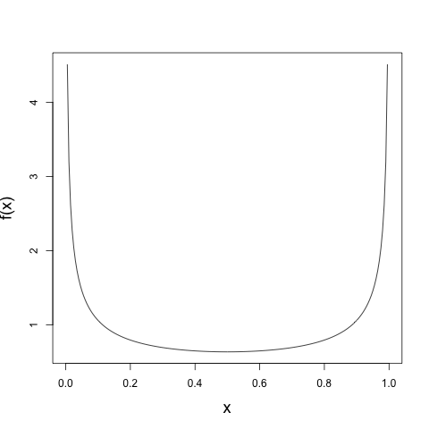
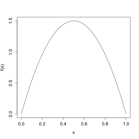
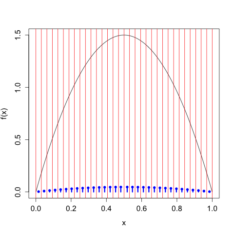
This is all well and good, but what does this discretization look like in practice? The text that I'm getting this from, Cover and Thomas's Elements of Information Theory, gives the example of \(X\) distributed according to various types of uniform and \(X\) distributed according to a Gaussian. The former is pretty boring (and has the disadvantage that the \(x_{i}\) we choose are not unique), and the latter would make for some annoying computation. Let's compromise and choose a density more interesting than a constant, but less involved than a Gaussian. We'll take \(X\) to have the density given by \[f(x) = \left\{\begin{array}{cc} 6 x (1-x) &: 0 \leq x \leq 1 \\ 0 &: \text{ otherwise} \end{array}\right.\] which is a friendly parabola taking support only on \([0, 1]\) and normalized to integrate to 1.

We'll take our discretization / bin width to be \(\Delta = 2^{-n}\), so we'll first divide up the interval into halves, then fourths, then eighths, etc. Since we know \(f(x)\), for each of these intervals we can apply the Mean Value Theorem to find the appropriate representative \(x_{i}\) in each \(I_{i}\). For example, here we take \(n = 2\) and \(\Delta = 1/2\):

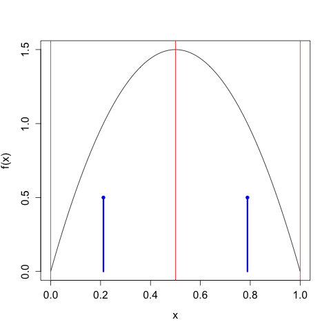
The red lines indicate the demarcations of the partitions, and the blue 'lollipops' indicate the mass assigned each \(x_{i}\). As expected, we choose two candidate points that put half the mass to the left of \(x = 1/2\) and half the mass to the right. All points to the left of \(x = 1/2\) get mapped to \(x_{0} = \frac{1}{2} - \frac{\sqrt{3}}{2} \approx 0.211\), all points to the right of \(x = 1/2\) get mapped to \(x_{1} = \frac{1}{2} + \frac{\sqrt{3}}{2} \approx 0.789\).

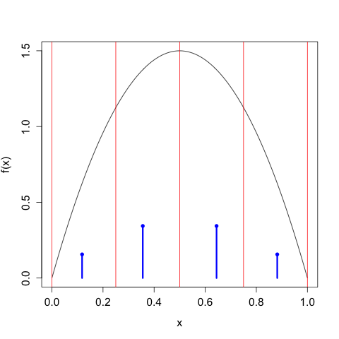
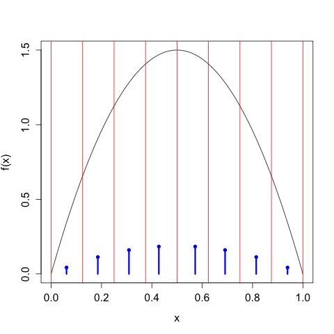
We can continue in this way, taking \(n\) larger and larger, and we get the following sequence of discretizations:

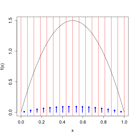
As we take our discretization to be finer and finer, the discrete entropy of \(X^{\Delta(n)}\) increases without bound, \[\begin{align} H\left[X^{\Delta(1)}\right] &= 1 \\ H\left[X^{\Delta(2)}\right] &= 1.896 \\ H\left[X^{\Delta(3)}\right] &= 2.846 \\ H\left[X^{\Delta(4)}\right] &= 3.828 \\ \vdots \\ H\left[X^{\Delta(4)}\right] &= 9.189, \end{align}\] We need to control this growth by tacking on the \(\log_{2} \Delta(n)\) term, in which case we have \[\begin{align} H\left[X^{\Delta(1)}\right] + \log_{2}(\Delta(1)) &= -1.110 \times 10^{-16} \\ H\left[X^{\Delta(2)}\right] + \log_{2}(\Delta(2)) &= -0.1039 \\ H\left[X^{\Delta(3)}\right] + \log_{2}(\Delta(3))&= -0.154 \\ H\left[X^{\Delta(4)}\right] + \log_{2}(\Delta(4))&= -0.172 \\ \vdots \\ H\left[X^{\Delta(10)}\right] + \log_{2}(\Delta(10))&= -0.1804, \end{align}\] which of course gets closer and closer to the differential entropy \(h[X] \approx -0.180470.\)

As usual, dealing with the continuum makes our lives a bit more complicated. We gain new machinery, but at the cost of our intuition.

In particular, because we have assumed that \(X\) admits a density, we know that \(f\) must be continuous, because otherwise it would not admit a density. For example, if it did have discontinuities, then probability mass would leave at those discrete points, and the density would not exist.↩

Poisson's Urns

I have been discussing the second half of Poisson's researches. Let us now turn to the first, and to the celebrated law of large numbers. The connection is that 'r', the 'average' reliability of a juror. Poisson's mathematical problem was well understood for situations which could be modeled with each juror having the same reliability as every other. But this, as Ostrogradsky had observed, is preposterous. Some jurors are more reliable than others. Poisson's law of large numbers was devised in order to solve just this problem. He studied as a model the situation in which reliability varies from juror to juror, but in which there is some law (Poisson's word) or probability distribution (our phrase) for reliability among French jurors.

Abstractly, the situation was this. Jacques Bernoulli's famous theorem, published posthumously in 1713, applied to repeated drawings, with replacement, of balls from an urn with black and white balls. Let the proportion of black balls in the urn be p. We take this to be the probability of drawing a black ball. Draw a ball, note its colour, replace it and shake the contents. We can consider a sequence of many such draws, and the relative frequency with which black is drawn on such a sequence. We can ask, what is the probability that the relative frequency is within some 'error' e of p? Bernoulli could answer, and that answer became well known. But suppose one is considering a population of urns in which the proportion of black balls varies from urn to urn? We choose an urn at random, and then draw a ball at random. Once again, in repeated urn/ball draws, there will be a relative frequency with which black is drawn. Let q be the overall proportion of black balls in the urns. Can we make any statement about the probability that the relative frequency of drawing black, in urn/ball selections, is within some small 'error' of q? Yes. The precise statement is what Poisson called the law of large numbers.

— Ian Hacking, from The Taming of Chance, p. 102

Let's see if we can get close to the result alluded to by Hacking. As usual, I'll start by being overly formal. By the end, we'll see a surprising (to me, at least) result about Poisson's ball and urn(s) problem.

Suppose we have a population of urns that we select from at random. For simplicity, we'll assume that we have a continuum of urns, and that the proportion of black balls in each urn is distributed uniformly on \([0, 1]\). Once we've chosen an urn, we'll draw a single ball from it, note its color, and then place it back into the urn. Then we'll choose a different urn at random, and continue in this way until we've noted the color of \(K\) urns. Because we have a continuum of urns where the success probabilities are uniform on \([0, 1]\), the overall proportion of black balls in the urns is just the expected value of this uniform distribution, namely \(1/2\). We are then asking: if we randomly select urns, and then randomly select balls from those urns, will the frequency of black balls converge on \(1/2\)?

Let \(P_{k}\) be the success probability for a given urn. We have already said that \(P_{k} \sim U(0, 1)\). Once we've chosen an urn, the probability of drawing a black ball is fixed at \(P_{k} = p_{k}\), and thus the outcome of the draw \(B_{k}\) is Bernoulli(\(p_{k}\)). We can summarize these relationships by saying \[\begin{align*} P_{k} &\sim U(0, 1) \\ B_{k} | P_{k} = p_{k} &\sim \text{Bernoulli}(p_{k}). \end{align*}\] And now we ask \[ \frac{1}{K} \sum_{k = 1}^{K} B_{k} \xrightarrow{???} E[P] = 1/2.\]

The answer is yes. And the quickest way to get there (that I've thought of) is to determine the marginal distribution of the \(B_{k}\). That is, we know the marginal distribution of \(P_{k}\), and we know the conditional distribution of \(B_{k}\) given \(P_{k}\). So we can append those two together to get the joint distribution of \((B_{k}, P_{k})\) and then marginalize out the \(P_{k}\) to get the marginal distribution of \(B_{k}\). I was surprised by the result, though perhaps should not have been.

Performing a few computations, we see that \[ f(b, p) = f(p) f( b | p) = 1 \cdot p^{b} (1 - p)^{1-b}\] and thus \[ f(b) = \int_{0}^{1} 1 \cdot p^{b} (1 - p)^{1-b} \, dp.\] At this point, we could brush off our NIST Digital Library of Special Functions and look up the Beta function. Or we can take note that we only care about when \(b = 0\) (which gives us the probability of seeing a white ball) or \(b = 1\) (which gives us the probability of seeing a black ball). For example, substituting in \(b = 1\), we get \[ f(1) = \int_{0}^{1} 1 \cdot p \, dp,\] which is just the expected value of \(P\), namely 1/2. Thus, we see that the \(B_{k}\) are marginally Bernoulli(\(E[P]\)). Of course, after we've seen this trick with \(P \sim U(0, 1)\), we notice that we can pull the same trick for \(P\) distributed according to any well-behaved distribution. This is because we'll always have \[ f(1) = \int_{S(P)} f(p) \cdot p \, dp = E[P],\] where \(S(P)\) is the support of \(P\), namely \(S(P) \subset [0, 1]\), and in the original example, \(S(P) = [0, 1]\).

And this is the result that I found weird. We're choosing the success probabilities according to some distribution \(P\), and then choosing the balls based on this success probability. And yet marginally, if we just looked at the \(B_{k}\), they will look identical to if we just sampled the \(B_{k}\) according to a Bernoulli(\(E[P]\)) distribution. In other words, we might as well skip straight to sampling \(B_{k}\) instead of first sampling \(P_{k}\) and then sampling \(B_{k} | P_{k} = p_{k}\). It wasn't obvious to me that this should be the case. And yet that is what's going on. Even if we take \(P\) to be discrete. For example, if we have ten urns, each with a different proportion of black balls, and we choose each urn with equal (or for that matter, unequal) probability. On each draw, it will be precisely as if we've sampled from a single urn with the proportion of black balls given by the (possibly weighted) average over the proportions from all of the urns.

And now Poisson's result is straightforward to show. We can apply either the weak or strong law of large numbers directly to the sequence \(B_{1}, B_{2}, \ldots\) and we get what we want. Namely, \[ \frac{1}{K} \sum_{k = 1}^{K} B_{k} \xrightarrow[\text{or } a.s.]{P} E[P] = 1/2\]

So Poisson's problem really reduces to Bernoulli's problem, if we look at it in the right way.

Levitt and the Language of Science

So for instance, after we published Freakonomics, some of my colleagues were not that wild about the book and the attention we received. So to try to shame me, one of my colleagues put up anonymously on the bulletin board for the department of economics a supposed quote from me that said, they claimed that I had said that, "Mathematics was not required to understand reality." Right? And this was supposed to be the most shameful, embarrassing quote. And the idea was that if it was known publicly that I had said this that it would ruin my reputation and I would feel awful about myself. But in fact it had just the opposite effect because I don't think mathematics is necessary to understand reality, and indeed I took tremendous satisfaction from the idea that I stood apart from the profession in believing this thing, which I think is obviously true. So while the intention of the act was to shame me, I've still got that sign up in my office. And I get utility out of it every single day when I walk in and I see it.

— Steven Levitt, excerpted from here

I remember hearing this quote in the Freakonomics podcast. I seem to recall thinking that Levitt misspoke, and couldn't possibly mean what he said.

Reading the quote again now, I'm uncertain if Levitt is being intentionally misleading, or if he has convinced himself of the case. Levitt is an economist. That means, most likely, that large parts of his research rely on regression (probably of the linear variety, but I'll give him the benefit of the doubt and assume he uses things like additive models. This work falls under the name 'econometrics,' which is economist slang for statistics. Which means it relies heavily on mathematics.

Of course, Levitt may be claiming that he can get by using these tools without understanding them. That would at least represent an honest statement. It probably wouldn't be good for his credibility or his career, but it would be honest. I also doubt that a Harvard and MIT educated economist doesn't understand basic regression.

Levitt tends to take the contrarian viewpoint on a lot of topics, sometimes because of temperament and sometimes because of the facts. But in this case, he is being intentionally misleading.

Math as Incantation

Our department recently hosted a series of talks by graduate and undergraduate students. I managed to participate¹ in the graduate student portion. I gave a mini-rant on the overuse of the phrase 'big data' (even though I included it in my title), and then presented a gentle introduction into computational mechanics. Overall, presenting was a very positive experience. I tried to follow some best practices, despite my crippling monotone.

The undergraduates spoke as part of the Math departments Directed Reading Program. We had a good mix of topics: variational calculus, compressive sensing, the algebra of the Rubik's cube, the list goes on. The beauty of studying mathematics is that everyone can do something completely different. And they all did an amazing job. They would have blow undergraduate-me away.

It was interesting viewing undergraduate presentations from the perspective of a graduate student. I've traced my first undergraduate presentation to a course titled, appropriately, Effective Communication for Chemists. I talked about evolutionary psychology and theories positing that the human mind evolved to its current greatness so that guys and gals could get laid. As you do when you're a sophomore in college.

Thinking back on my undergraduate career, I gave very few talks. At least, in comparison to the three years I've now spent in graduate school. Part of that is because of the Scientific Computing project course sequence. But also just the new desire to share cool new ideas with others.

While watching the undergraduate talks, I noticed something weird. A lot of the students, especially the freshman, would take to reading equations off their slides, almost as an incantation. For example, in a talk about Black-Scholes, they might have a slide with the following expression:

\[ \frac{1}{\sigma \sqrt{T - t}} \left[ \log \left( \frac{S}{K} \right) + \left( r + \frac{\sigma^{2}}{2} \right) (T - t) \right]\]

Never mind what any of this means². In a graduate talk, we would speak around this expression. We might point out some key terms, to give a flavor, but we would never just read out the expression.

But a few of the undergraduates did this. Which, in retrospect, seems only natural. After a decent amount of training, you start to see a mathematical expression as a whole. But until then, you have to look at it a piece at a time, so it only seems natural that this is how you should present it to your audience.

The students who took this approach clearly knew what they were talking about. But they hadn't developed the fluency, or trust in our fluency, to skip past the phonics approach and embrace a whole language approach.

I wonder at what point in ones education that leap occurs? I certainly don't recall when it happened for me, but I know it must have.

Fortunately, this is entirely different from the cargo cult mathematics that I often see practiced. That's an entirely different 'mathematics as incantation.' None of the talks this year suffered from that. Which I take a very good sign of health for our department.

This presentation will not stand alone. But I take that as a point of pride with my talks. So... Good?↩
If you want to learn how to ruin the economy, you can read more here.↩

Black box algorithms are not enough

But, contrary to the message sent by much of Andrew Ng's class on machine learning, you actually do need to understand how to invert a matrix at some point in your life if you want to be a data scientist. And, I'd add, if you're not smart enough to understand the underlying math, then you're not smart enough to be a data scientist.

I'm not being a snob. I'm not saying this because I want people to work hard. It's not a laziness thing, it's a matter of knowing your shit and being for real. If your model fails, you want to be able to figure out why it failed. The only way to do that is to know how it works to begin with. Even if it worked in a given situation, when you train on slightly different data you might run into something that throws it for a loop, and you'd better be able to figure out what that is. That's your job.

— Cathy O'Neil from Statisticians aren't the problem for data science. The real problem is too many posers.

This post was in response to Cosma Shalizi's incredibly articulate argument that 'data science' is code for 'computational applied statistics.' That post is also definitely worth reading.

I've noticed this separation between the ability to use a tool and the ability to understand how it works in the courses I've TA-ed at Maryland. All of them¹ had a computational component, namely MATLAB. A very simple example immediately comes to mind: students did not understand the difference between an analytical solution to a differential equation and a numerical solution to a differential equation, or that, in fact, we sometimes can't find analytical solutions and have to fall back on numerics. The layout of the MATLAB assignments is largely at fault here. The assignments begin with MATLAB's Symbolic Toolbox (which I'm pretty sure no real researcher would ever use, compared to, say, Maple or Mathematica) instead of starting with the numerics (routines like ode45, the workhorse of MATLAB's numerical ordinary differential equation solvers). This is a necessary evil, I guess, but even by the end of the course I'm still not sure the distinction has sunk in.

This is a weird sort of situation, and a new one. It used to be that the only people who used computers also happened to be the ones who created them. And you damn well better believe they knew how to invert a matrix. There's something to be said for the democratization of algorithms. I think it's a good thing that the general public can do a massive eigenvalue problem every time they use Google without batting an eye. But that's the general public, not the scientists and engineers.

Now we have large segments of the scientific workforce who use computers (and the algorithms associated with them) as black boxes. I've heard many of my students say without batting an eye, "Why do I need to learn this? I'm just going to run a program on a computer at my job." I can't put myself in the headspace that finds that situation okay, and I suppose that goes a long way towards explaining why I'm in graduate school for applied mathematics and not working at an engineering firm somewhere.

This also reminds me of a conversation I had yesterday with a friend taking a course in computational neuroscience. At the end of the course, all of the students have to present a project that ideally incorporates material learned from the course. The year I took the class (two years ago, now!), and apparently this year as well, a lot of people completed the following 'project.' First, collect large amounts of data. Then perform Principal Component Analysis on that data to reduce the dimension of the data set. Finally, present the first few principal components, without any discussion of what they might mean beyond the fact that they account for such and such amount of variance. As if this means anything. Nevermind that principal component analysis only really makes sense when you're dealing with data that can be well-approximated by a multivariate Gaussian. This process of plugging data into an algorithm (that you don't even understand) and reporting the output is not science. What did you want to learn from your experiment? What question are you even asking? The democratized methods cannot get you to ask these important questions. And to the uninitiated, just saying that you did PCA can make you sound impressive. (Replace PCA with SVM, LDA, or any of various other acronyms that people find so impressive.)

I suppose I could be celebrating that in large parts of science it's so easy to get by without doing much science. But one of my biggest fears (at least career-wise) is spending a life doing crap science that no one cares about. I don't just want to get by. I want to contribute something worthwhile.

Except for STAT400, which, honestly, really should have had a computational component. Teaching statistics without playing around with pseudorandom numbers, especially for a course named Applied Probability and Statistics, is outrageous.↩

Flashcards

Anyone who has been in a class with me in graduate school knows that I'm a huge fan of flashcards. Well, really of spaced repetition for learning. The basic idea, first introduced to me in this Wired Magazine article, is very simple: we retain information best when space our exposure to it so that the time between exposures increases each time. For example, you might first require exposure to the idea immediately after learning it, then an hour later, then a day later, then a week later, etc. Any other spacing would be suboptimal, and would require either more time learning the material than is necessary, or would result in less material retained. Steven Strogatz and some others did a neat analysis of this problem from an abstracted perspective.

This puts a lot of responsibility on the part of the learner to figure out a system for when to review a card. Fortunately, a lot of software is already out there that automates this process. Some open source options include Mnemosyne and Anki. I use Mental Case.

I first learned about this approach the summer between my sophomore and junior year¹. I immediately put the system to use. My first flashcard in the system asked, "What are Maxwell's equations?" One of my more recent flash cards asks, "To show that the estimator from Maximum Likelihood Estimation is consistent (converges to the correct value of \(\theta\)), is the result that the negative mean log-likelihood converge (in probability or almost surely) to a function whose maximum is the true parameter value enough?" (The answer is no. You need the convergence to be uniform in \(\theta\).) This gives you a flavor of how my interests have changed over time.

I used (and continue to use) that system for studying since my junior year of college. I've created notes for every class I've taken since then, and have now started making notes as I go off learning material on my own. I have 3546 notes in my collection currently, though some of them are 'completed' (I'll never see that Maxwell's equations card again, and to be honest, don't remember them anymore). I can't prove that they've cut down on the number of hours I spent studying, but I do know that after I started using them, I no longer had extended study sessions before exams. I spread all of the studying out over the course of the semester, and then beyond. This also gives me an easily searchable repository of all the results I've ever learned. I've found myself going back to it more times than not when I have a result on the tip of my mind, but can't quite grasp it.

I recently read a post by Rhett Allain at Dot Physics where he flatly states that he's not a fan of flashcards. Of course, his conception of flash cards and mine couldn't be further apart. I use flashcards as an excuse to commit concepts to memory (recently, they've been the only reason I go back over notes that I've written), and as a crutch to keep those concepts on the top of my mind. Rhett has in mind rote memorization of facts just to get past an exam. I've been so far removed from that world that it's hard to imagine returning to it. That's one nice thing about being a (pseudo-)mathematician. Results follow naturally from the definitions we set up.

Here's my comment on Rhett's blog. Hopefully I come off less as an ass and more as someone offering constructive criticism.

In mathematics, at least, I've found flash cards to be an invaluable tool. (Well, spaced repetition software like Mental Case.) Large parts of mathematics begin with simple definitions, which we then build on to develop the theory. But if we don't even know the most basic definitions, how can we hope to scale to the heights of the theory?

At least in my process, definitions come first, and then understanding. If I can't state what some mathematical object is, then I have no hope of having any intuition about it. During the courses I've TAed as a graduate student, I've stressed this fact with my students. Especially in a definition-heavy course like linear algebra. They have to know what it means for a collection of vectors to form a basis (i.e. a basis is a linearly independent spanning set for some vector space) before they can begin to get the intuition for what that means (a basis gives you a way of labeling all points in a vector space).

An anecdote about Feynman related to the "couldn't you just look this up online?" point:

'Richard Feynman was fond of giving the following advice on how to be a genius. You have to keep a dozen of your favorite problems constantly present in your mind, although by and large they will lay in a dormant state. Every time you hear or read a new trick or a new result, test it against each of your twelve problems to see whether it helps. Every once in a while there will be a hit, and people will say, "How did he do it? He must be a genius!"'

You can't make a connection unless you have the basic facts behind the connection readily at hand.

Admittedly, I probably use flashcards very differently from what you have in mind with this post. The notes I write for myself are much more about the concepts than any particular mathematical expression (though I try to keep those fresh, too). And I actively think about each note when I review ("Why is the expression this way and not that?", "What would happen to this theorem if we tried to weaken this assumption?", etc.), rather than perform rote memorization.

I've had thoughts of posting my flashcards online at some point. But I think they may be so tailor made to my own use that they don't be useful to others.

That was my 'summer of the chemist,' when I attended a REU at Texas A&M under the advisement of Dave Bergreiter. I studied solute effects on PNIPAM, poly(N-isopropylacrylamide). That was also the summer when I learned that, unlike my brother, I would never be a synthetic chemist. Probably all for the better.↩

Simulating Randomness

I've just started watching the lectures of Jim Crutchfield for his course Natural Computation and Self-Organization at UC Davis. These lectures are the closest thing to a textbook for the discipline of computational mechanics, and I need to brush up on some details before my preliminary oral exam sometime this summer.

During the first lecture for the second half of the course (it's broken up into 'Winter' and 'Spring' halves), Jim points out that nature finds uses for randomness. This immediately reminded me of my recent post where I found a (trivial) use for randomness in a simple rock-paper-scissors game. In his lecture, Jim also pointed out that we now know simple ways of generating pseudo-random numbers using deterministic processes. Namely, chaos.

This immediately sent me down a rabbit hole involving the logistic map, everyone's favorite example of a one-dimensional map that, for certain parameter values, can give rise to chaos. For the uninitiated, here's the map:

\[ x_{n+1} = r x_{n}( 1 - x_{n}) \]

where \(r\) is a positive parameter. This very simple discrete map (it's only a first-order nonlinear difference equation, after all) can lead to chaotic dynamics for values of \(r\) greater than some critical value \(r_{c}\)¹. And chaotic systems can look random, at least random enough for most purposes, if you don't know their governing equations. For example, here's 1000 iterations from the logistic map when \(r = 4\):

That looks pretty random. Of course, if you were to rerun my code, using exactly the same initial condition I did, you would get exactly the same iterates. It is deterministic, after all.

Which brings me back to Jim's point about nature finding ways to harness chaotic systems to generate pseudo-randomness. Developing one's own pseudo-random number generator can be a fool's errand², but if you can get something that generates numbers that look like independent draws from a distribution uniform on the interval from 0 to 1, then you're off to the races. These sorts of samples are the building blocks for methods that sample from more interesting distributions, methods like Metropolis-Hastings and Gibbs sampling.

Fortunately, mathematicians far smarter than I (Ulam and von Neumann come to mind) have figured out some properties about the logistic map when \(r = 4\) that I can use to my advantage. For one thing, the natural measure of the logistic map has a density given by \[ f(x) = \left \{ \begin{array}{ll} \frac{1}{\pi \sqrt{x(1-x)}} & : x \in [0, 1] \\ 0 & : \text{ otherwise} \end{array}\right .,\] which if we plot on the interval \([0, 1]\) looks like

The meaning of the natural measure for a dynamical system would require a bit more theory than I want to go into here. But here's the intuition that Ed Ott gave in his chaotic dynamics class. Sprinkle a bunch of initial conditions on the interval \([0, 1]\) at random. Of course, when we say 'at random,' we have to specify at random with respect to what probability measure. The natural measure of a dynamical system is the one that, upon iteration of initial conditions sprinkled according to that measure, results in a measure at each future iteration that hasn't changed. You can think of this as specifying a bunch of initial conditions by a histogram, running those initial conditions through the map, and looking at a histogram of the future iterates. Each initial condition will get mapped to a new point. But each new histogram should look the same as the first. In a sense, we can treat each iterate \(x_{n}\) of the map as if it were drawn from a random variable \(X_{n}\) with this invariant measure.

Clearly, the invariant measure isn't uniform on \([0, 1]\). We'll have to do a little bit more work. If we can treat the iterates \(x_{1}, x_{2}, \ldots, x_{n}\) as though they're random draws \(X_{1}, X_{2}, \ldots, X_{n}\) from the distribution with density \(f\), then we have a way to transform them into iterates that look like random draws \(U_{1}, U_{2}, \ldots, U_{n}\) from a distribution uniform on \([0, 1]\). The usual trick is that if \(X\) has (cumulative) distribution function \(F\), then \(U = F(X)\) will be uniform on \([0, 1]\). That is, applying the distribution function that governs a random variable to itself results in a uniform random variable. We can compute the distribution function for the invariant measure in the usual way, \[ \begin{align*} F(x) &= \int_{-\infty}^{x} f(t) \, dt \\ &= \int_{0}^{x} \frac{1}{\pi \sqrt{t(1-t)}} \, dt \end{align*}.\] After a few trig substitutions, you can work out that the distribution function is given by \[ F(x) = \left \{ \begin{array}{ll} 0 & : x < 0 \\ \frac{1}{2} + \frac{1}{\pi} \arcsin(2x - 1) & : 0 \leq x \leq 1 \\ 1 & : x > 1 \end{array}\right . .\]

Plotting this on the interval \([0, 1]\), we get

where the blue curve is the true distribution function and the red curve is the empirical distribution function inferred from the thousand iterates. So if we compute \(u_{n} = F(x_{n})\) for each iterate, we should get something that looks uniform. And we do:

So, the theory works. We've taken a dynamical system that should behave a certain why, and transformed it so that it will look, for the purpose of statistical tests, like draws from a uniform distribution. Here's the transformed iterates:

and a draw of 1000 variates using R's runif³:

Both look pretty random. But there's a fatal flaw in this procedure that would make any cryptoanalyst blush. Remember that the iterates were generated using the map \[ x_{n+1} = r x_{n}( 1 - x_{n}).\] This means that there is a deterministic relationship between each pair of iterates of the map. That is, \(x_{n+1} = M(x_{n})\). We've applied \(F\) to the data, but \(F\) is a one-to-one mapping, and so we also have \(u_{n + 1} = F(M(x_{n})) = H(u_{n})\). In short, if we plot \(u_{n}\) vs. \(u_{n + 1}\) for \(n = 1, \ldots, 999\), we should get something that falls on the curve defined by \(H\). And we do:

If the iterates were truly random draws from the uniform distribution, they should be spread out evenly over the unit square \([0, 1] \times [0,1]\). Oops. Instead, we see that they look like iterates from another simple dynamical system, the tent map. This is no coincidence. When \(r = 4\), iterates from the tent map and the logistic map are related by the function \(F\), as we've just seen. They're said to be conjugate.

So this is no good, if we want to use these pseudorandom numbers to fool someone. Which got me to thinking: can we combine two deterministic sources to get something that looks random? The process is simple. Generate two sequences of length \(n\) using the logistic map with different initial conditions. Call these \(x_{1}^{(1)}, \ldots, x_{n}^{(1)}\) and \(x_{1}^{(2)}, \ldots, x_{n}^{(2)}\). Map both sequences through \(F\), giving two draws \(u_{1}^{(1)}, \ldots, u_{n}^{(1)}\) and \(u_{1}^{(2)}, \ldots, u_{n}^{(2)}\) that look, except for the recurrence relation above, like random draws from a uniform distribution. Now sort the second sequence from smallest to largest, keeping track of the indices, and use those sorted indices to shuffle the first sequence. That is, compute the order statistics \(u_{(1)}^{(2)}, \ldots, u_{(n)}^{(2)}\) from the second sequence (where those order statistics will still look random, despite the recurrence relation), and use those to wash out the recurrence relationship in the first sequence. If we plot these iterates against each other, as before, we get what we would hope:

Of course, I still wouldn't recommend that you use this approach to generate pseudorandom numbers. And I imagine that other methods (like the Mersenne Twister referenced in the footnotes) are much more efficient. But it is nice to know that, if stranded on a desert island and in need of some pseudorandom numbers, I could generate some on the fly.

What else would I do with all that time?

The term 'chaos' means two very different things to specialists and the general public. I'll point you to a post I made on Quora that gives my working definition.↩
To quote the professor from my first year scientific computing course: "Pseudo-random number generators for the uniform distribution are easy to write but it is very, very difficult to write a good one. Conclusion: don't try to write your own unless you have a month to devote to it."↩
R, Python, and MATLAB (the three major scripting languages used in scientific computing) use a much more sophisticated algorithm called the Mersenne Twister. We'll see why we need something more sophisticated in a moment.↩

LaTeX — Necessary but Not Sufficient

Whenever I read papers with mathematical content not written in LaTeX, I immediately judge the content. Usually to be lacking. I know I shouldn't do this. But previous experience has shown this to be a useful heuristic.

What do I mean? For those outside the mathematical community, LaTeX is a mathematical typesetting language. You can think of it like a markup language (similar to HTML), but for making documents with lots of mathematics. Donald Knuth created TeX in 1978. HTML was created in 1990.

LaTeX is one of those things that you hate at first, then begin to tolerate, and eventually come to love. At least, that's been my trajectory.

And once you do start to love it, it becomes a shibboleth¹ that separates the mathematically knowledgeable from those who, well, aren't².

Here's a recent example from the arXiv: On the distribution of time-to-proof of mathematical conjectures³. This sounds like a cool idea. And the data the authors gathered probably took some time to collect. But then the analysis goes off the rails.

I won't go through how. I'll leave that as an exercise for the reader.

But the point is that the paper wasn't written in LaTeX. Much like this paper on how life predates earth⁴. Spoiler alert: if it does, this analysis certainly doesn't show it.

Aside: I should really start publishing things to the arXiv. If these papers are on there...

Much like lower case xi.↩
Admittedly, LaTeX is a necessary but not sufficient condition for a contentful paper. Take this amusing, but scientifically content-less, paper on zombie models. Beautifully typeset, but not likely to make a major contribution to the greater body of scientific knowledge.↩
And then I learned the authors are from ETH Zurich's Department of Management, Technology and Economics. Okay, that makes a lot more sense.↩
Leave it to the Huffington Post to take this story seriously. Then again, I'll hope people don't get their science news from the Huffington Post... But so did the Physics arXiv Blog. Oh...↩

Rock, Paper, Scissors… Random!

First, watch this video. It's a talk (really more of a chat) by Jad Abumrad of Radiolab¹ fame.

Done watching? Then you don't need me to tell you Jad, in part, discusses the uses of randomness in nature. Here's a favorite quote of mine:

What they basically saw is the randomness of biology guiding behavior. Now you could try and explain this randomness away, and people have. And certainly this is speculative what I just said. But essentially what they saw was that the monkey's — the latent stochastic chaos in the monkey's brain was contributing to an effective rock-paper-scissors strategy. Because you have to be unpredictable!

"You have to be unpredictable!" The line about a rock-paper-scissors strategy got me to thinking of this little game the New York Times threw together: Rock-Paper-Scissors: You vs. the Computer. Okay, they didn't invent the game. But they did think to use some statistical analysis of human rock-paper-scissors behavior to find a winning strategy. As they warn in the text:

Computers mimic human reasoning by building on simple rules and statistical averages. Test your strategy against the computer in this rock-paper-scissors game illustrating basic artificial intelligence. Choose from two different modes: novice, where the computer learns to play from scratch, and veteran, where the computer pits over 200,000 rounds of previous experience against you.

Note: A truly random game of rock-paper-scissors would result in a statistical tie with each player winning, tying and losing one-third of the time. However, people are not truly random and thus can be studied and analyzed. While this computer won't win all rounds, over time it can exploit a person's tendencies and patterns to gain an advantage over its opponent.

I'll repeat the key line, because it loops back around to Jad's comment above:

However, people are not truly random and thus can be studied and analyzed. While this computer won't win all rounds, over time it can exploit a person's tendencies and patterns to gain an advantage over its opponent.

Try playing a few rounds. I'll wait.

Back? Did you win?

I did. And my 'strategy' was simple: be random. If you understand how the computer chooses its moves, it becomes very easy to beat. Here's one run of 150 trials with the computer on veteran:

As you can see, I won. Not by a large margin. But if I kept playing, the proportions of wins/ties/losses would stabilize, and not to (1/3, 1/3, 1/3).

Why? Because my strategy was this:

numpy.random.randint(3, size = 150)²

array([0, 2, 1, 2, 2, 1, 2, 0, 1, 2, 2, 0, 1, 2, 1, 0, 2, 1, 0, 2, 2, 0, 2, 1, 2, 0, 0, 0, 1, 1, 2, 0, 0, 0, 2, 0, 1, 2, 0, 2, 1, 2, 0, 2, 0, 0, 2, 0, 2, 0, 1, 2, 0, 2, 0, 1, 2, 2, 1, 1, 2, 0, 2, 0, 2, 0, 2, 1, 0, 0, 1, 1, 0, 1, 1, 1, 0, 0, 2, 1, 2, 1, 1, 2, 2, 1, 1, 2, 2, 1, 1, 1, 1, 2, 1, 1, 2, 2, 2, 0, 0, 1, 1, 1, 0, 0, 1, 1, 0, 1, 1, 0, 0, 0, 0, 1, 0, 1, 2, 0, 0, 2, 0, 0, 1, 2, 2, 1, 0, 0, 0, 2, 2, 2, 2, 1, 0, 0, 2, 0, 0, 1, 0, 0, 2, 2, 1, 2, 1, 2, 2, 1, 1, 2, 2, 0, 1, 0, 2, 2, 2,...

Basically, I sampled 150 draws from a uniform distribution over the values {0 (rock), 1 (paper), 2 (scissors)}. And then played those values out. Humans are bad at simulating randomness. But computers aren't. And using this strategy, you too can outperform the computer.

The New York Times explains why in their demo. As they say in the header text, 'the computer pits over 200,000 rounds of previous experience against you.' If you walk through their tutorial, they explain what this mean. Basically, they infer a Markov model of sorts. "What is the probability that Dave throws \(x\) given that in the three previous rounds, he threw \((d_1, d_2, d_3)\), and in the three previous rounds, I threw \((c_1, c_2, c_3)\)?" You can infer this probability using statistics (via maximum likelihood estimation, if they're smart), and predict my next move as the argument \(x\) that maximizes the conditional probability \(p(x | (d_1, d_2, d_3), (c_1, c_2, c_3))\). You'll infer a bunch of transition probabilities, and using those you can try to beat me.

But the computer was playing against people, not random number generators. Thus, the probabilities inferred don't agree with the new data-generating distribution (me, or really my random number generator), and so the algorithm does terribly. The learning method they use doesn't generalize to new data. Offline learning algorithms tend to do terribly with non-stationary distributions.

There are ways to get around this. A popular approach within the field of machine learning is online learning. This is aptly named, because you try to learn the data generating process as you go. This is a cool book on the topic that I'll have to add to the long list of textbooks I'd like to study.

If you'd like to play along at home, you can get out your favorite six-sided die and go to town beating the computer. It won't mind.

What's that? You don't listen to Radiolab? Shame on you. Stop reading this post and listen to one of their podcasts right now!↩
And randomness is a limited resource!↩

Berry-Esseen Deserves More Praise

Everyone knows the Central Limit Theorem¹. In the simplest case, the theorem says that for independent draws from a population that is 'sufficiently well-behaved,' the probability statements that you can make about the sample mean converge, in the limit, to the probability statements you can make about a normal random variable with a mean given by the population mean and a variance given by the population variance over \(n\), the number of data points in your sample. In slightly gorier detail, if we have a sample of independent and identically distributed random variables \(X_{1}, \ldots, X_{n}\) with each having mean \(E[X] = \mu < \infty\) and variance \(\text{Var}(X) = \sigma^{2} < \infty\), then \[\frac{1}{n} \sum_{i = 1}^{n} X_{i} \xrightarrow{D} Y \sim N(\mu, \sigma^{2}/n).\]

This is a very nice theorem. It says that no matter what distribution the \(X_{i}\) have, as long as it's not too pathological², the sample mean can be treated like a normal random variable for probabilistic computations. And in statistics, these are the sorts of statements we'd like to make.

This may seem weird. At least, it seemed weird to me the first time I heard it. What if I take the average of a bunch of Uniform(0, 1) random variables? That is, take a bunch of random variables sampled from the unit step function on \([0, 1]\), and take their average. That starts out decidedly non-normal. But in the limit, you get something that looks³ normal.

The flat curve, horizontal at 1, is the density of a uniform random variable. Each successive curve is the density of \(\bar{X}_{n}\) for larger and larger values of \(n\), going up to 19. As we'd expect, if you average a bunch of numbers between 0 and 1, their average stays between 0 and 1. But we see that, as the central limit theorem promises, the average becomes more and more normal, going from a triangular density at \(n = 2\) to something nearly indistinguishable from a normal density at \(n = 19\). Also as promised, the density becomes more and more concentrated around the true expected value, in this case \(1/2\), as the variance decreases like \(n^{-1/2}\).

This is all standard fair in any introductory statistics course⁴. What is less standard is the statement about how quickly the sample mean converges to a normal random variable. Asymptotics are nice, but they're, well, asymptotic. Usually we only have a finite amount of data. It would be nice if we could make a statement about how well the \(N(\mu, \sigma^{2}/n)\) approximation works for \(n\) much less than infinity.

And it turns out that we can. The result that gives us the statement is the Berry-Esseen Theorem. Larry Wasserman first brought this result to my attention in his post here. Which, come to think of it, is the first time I saw the theorem stated. I could have sworn I'd also seen it in his All of Statistics, but the theorem isn't in the index.

Without further adieu, here's the theorem.

Theorem: (Berry-Esseen)

Let \(X_{1}, \ldots, X_{n}\) be iid with finite mean \(\mu\) and finite variance \(\sigma^{2}.\) Define

\[Z_{n} = \frac{\sqrt{n} (\bar{X}_{n} - \mu)}{\sigma}\]

Then

\[\sup_{t} |P(Z_{n} \leq t) - \Phi(t)| \leq \frac{0.4784 \beta_{3}}{\sigma^{3} \sqrt{n}},\]

where \(\Phi\) is the standard normal cdf and \(\beta_{3} = E[|X_{i}|^3]\)

There's a lot to chew on here, and it's worth going through the theorem and trying to unpack the consequences for yourself⁵. But being a bit hand-wavy, it says that if you make a probabilistic statement⁶ using the normal approximation, for any \(n\) you'll be off at most \(\frac{0.4784 \beta_{3}}{\sigma^{3} \sqrt{n}}\) from if you used the actual sampling distribution of the sample mean for the underlying distribution⁷. Since we don't usually know the parameters of the true population, let alone the type of distribution, this is a comforting result. Unless the \(\beta_{3}\) term is very large, we won't do so bad in using this approximation: our error goes down like \(n^{-1/2}\). And we can do all sorts of things with this approximation: perform hypothesis tests, construct confidence intervals, you name it.

We see from this result that the appropriate way to compare the sampling distribution of the sample mean and the normal approximation is through their cumulative distribution functions. Here's the comparison for \(n = 5\) for the sample mean from a uniform distribution:

You'll have a hard time telling the difference from this plot, unless you have a really good eye. The help out, here's the absolute error between the true sampling distribution and the normal approximation as a function of \(t\):

We see that even at the worst \(t\), we don't do worse than a difference of 0.007. That's pretty good. Especially considering that the upper bound from the theorem says we'll have error at most 2.20. (We do better than this, which is okay with an upper bound.)

I'll finish with a quote from the book Numerical Recipes⁸, to remind us what the Central Limit Theorem does and doesn't state, and how people can misunderstand it:

For a hundred years or so, mathematical statisticians have been in love with the fact that the probability distribution of the sum of a very large number of very small random deviations almost always converges to a normal distribution. [...] This infatuation tended to focus interest away from the fact that, for real data, the normal distribution is often rather poorly realized, if it is realized at all. We are often taught, rather casually, that, on average, measurements will fall within +/-\(\sigma\) of the true value 68% of the time, within +/-2\(\sigma\) 95% of the time, and within +/-3\(\sigma\) 99.7% of the time. Extending this, one would expect a measurement to be off by +/-20\(\sigma\) only one time out of \(2 \times 10^{88}\). We all know that "glitches" are much more likely than that!

— W.H. Press et al., Numerical Recipes, Sec. 15.1

I don't know what Press means by 'almost always' (statements like 'almost always' and 'almost surely' mean something very particular in probabilistic contexts). And it sounds like Press had a pretty poor statistics professor, or more likely never took a real course in a statistics department. He makes the mistake I warned against in the footnotes: don't conflate the fact that you can make approximately normal statements about the sample mean with the population being normal. No mathematical statistician thinks that.

That said, here's my response from October 2012:

I don't think it's fair to blame the mathematical statisticians. Any mathematical statistician worth his / her salt knows that the Central Limit Theorem applies to the sample mean of a collection of independent and identically distributed random variables, not to the random variables themselves. This, and the fact that the \(t\)-statistic converges in distribution to the normal distribution as the sample size increases, is the reason we apply any of this normal theory at all.

Press's comment applies more to those who use the statistics blindly, without understanding the underlying theory. Which, admittedly, can be blamed on those same mathematical statisticians who are teaching this very deep theory to undergraduates in an intro statistics class with a lot of (necessary at that level) hand-waving. If the statistics user doesn't understand that a random variable is a measurable function from its sample space to the real line, then he/she is unlikely to appreciate the finer points of the Central Limit Theorem. But that's because mathematical statistics is hard (i.e. requires non-trivial amounts of work to really grasp), not because the mathematical statisticians have done a disservice to science.

Earlier inklings of my railing against the 'statistical-industrial complex.'

Actually, I didn't know Wikipedia has such a nice demonstration of the Central Limit Theorem in action. It puts what I'm about to do to shame.↩
For an example of a 'pathological' random variable, consider the Cauchy distribution. The sum of independent Cauchy random variables is Cauchy, so we have no hope of ever getting a normal random variable out of this limiting process. Oh, and the mean and variance of a Cauchy random variable are not defined.↩
This figure took a surprisingly long time to make. I had to remind myself about convolutions and the Fast Fourier Transform. Fortunately, as they often do, numerics saved me from a lot of tedious integrals.↩
Standard, and yet I imagine very misunderstood. I might be projecting myself onto my students, but I just always had the hunch that they didn't really know what this theorem is saying. For example, here's a common misconception that I might have projected: "The population becomes normal." No, the fact that we don't need that is precisely the power of the Central Limit Theorem.↩
In fact, this sort of 'unpacking' is the type of thing that separates your average undergraduate from your average graduate student. Or, How to Read Mathematics.↩
We make probability statements with cumulative distribution functions, and this is what both \(P(Z_{n} \leq t)\) and \(\Phi(t)\) are, the things we're computing the distance between.↩
Curious about the constant (0.4784)? Read the Wikipedia article to learn about the hard fought struggle to bring it down from its start at 7.59. These battles fascinate me. I wonder if people make careers out of these sorts of results (getting a tighter upper bound), or if most of them are one-off findings in a career spent on other things.↩
This is an interesting book. In graduate school, I've heard two very different perspectives on it. From the mathematicians, especially the numerical analysts, mostly distain. From the physicists, admiration. If the section I quote is any indication of the quality of the rest of the book, I think I'll have to side with the analysts.↩

DNA Sequences as a Stochastic Process

Occasionally I'll write a response to a question on Quora. Partly as a means to procrastinate, partly for educational purposes, and partly to 'show off.'

Here was my answer to the question Can DNA sequences be treated as timeseries?

A DNA sequence (ACGTACT..., for example) is a collection of bases that have a definite spatial order (the A really does precede the C, which really does precede the G, etc., in the DNA molecule, at least if we read the molecule linearly, from 5' to 3', for instance). Since the indexing matters, we have found ourselves in the realm of stochastic processes. A stochastic process (at least from one perspective) is an indexed collection of random variables. The simplest stochastic process that most scientists are familiar with is a random sample, the so-called IID (independent and identically distributed) stochastic process where each instance in the sequence is independent of each other instance, and all of the sequences have the same distribution. This is the bread and butter of introductory statistics courses (mostly because assumptions of IIDness make problems tractable). But nature need not behave according to our theories from STAT100.

A general stochastic process allows for arbitrary dependencies between all of the random variables. For instance, it might be the case that an A is more likely to follow a G (I don't know the biology, but I have seen evidence that this sort of thing does happen in real genomes), or a T to follow a C. If we incorporate this sort of information into our model of the DNA sequence, we have something called a first-order Markov chain (the probability of observing a base X only depends on the previous base observed, and is independent of all the bases before that). We can extend this to general nth order Markov chains, where the probability of observing a particular base only depends on the previous b bases (b = 1 gives us the first-order chain).

Another common stochastic process model used for DNA sequences is the Hidden Markov Model (often abbreviated HMM). In this case, we have a joint process, a symbol sequence that we do observe (in this case, the bases), and an unobserved 'state' sequence that we do not observe (but would like to infer). This is a common technique for identifying genes within a DNA sequence, where the hidden state transitions between 'gene' and 'not-gene'.

These ideas as applied to DNA sequences are old, dating back at least until the 1980s. See for example Gary Churchill's Stochastic models for heterogeneous DNA sequences (the first Google result for 'stochastic process DNA sequence').

Bringing things back around to the original question, a time series is just a particular type of stochastic process, where the index is over time. A DNA sequence is a very similar object, where the index is over space. In both cases, we are usually interested in the dependencies between nearby (and distant) observations, in time for time series and in space for DNA sequences. As such, the tools of one field can often be applied to the other. However, the tools of time series analysis usually involve real-valued observations (the closing price of the stock market on consecutive days, the weight of a patient over some period of time, etc.), whereas the observations of DNA sequences involve discrete observations from a fixed alphabet {A, G, C, T, U}. As such, we should be careful about any attempt to transplant tools directly from time series analysis to DNA sequence analysis.

The Bayesian Conspiracy

We started reading about Markov Chain Monte Carlo (MCMC, as the kids call it) in a statistics reading group I attend. In the process of learning the MCMC material, I have decided to actually learn some Bayesian inference techniques¹. I might write about the experience, though probably not. I can't imagine reading a generally pro-frequentist discuss the pros and cons of Bayesian methods would draw much of an audience. But I do have a few thoughts².

Learning this material reminded me of my first exposure to Bayes' Theorem. I first read about it in this post by Eliezer Yudkowsky. In the post, he presents a lucid discussion of using Bayes' theorem in a, at this point, standard situation. Suppose you have a test for a disease. The test has a 99.9% true positive rate. That is, the probability that the test is positive, given that you have the disease, is 99.9%. This leads most people (myself included, at times) to believe that if you test positive, you must have the disease. But this is getting the probability backwards. What we want to know is the probability that we have the disease, given that we test positive. In general, conditional probabilities aren't symmetric, that is \(P(B | A) \neq P(A | B)\), so we're asking the wrong question. There are two ways to handle the fact that we're asking the wrong question. Eliezer's method is to develop an intuition. His post does this very well, using numerical examples. As he claims,

While there are a few existing online explanations of Bayes' Theorem, my experience with trying to introduce people to Bayesian reasoning is that the existing online explanations are too abstract.

I'll take the 'too abstract' route, inverting Laplace's suggestion, "probability is nothing but common sense reduced to calculation," and hoping that we can refine our common sense by applying probabilistic rules. I won't go into all (or even most) of the details. But here's the setup. Let \(+\) be the event that you test positive for the disease. Let \(D\) be the event that you have the disease, and \(D^{c}\) be the event that you don't have the disease. Then Bayes' magical formula is just:

\(P(D | +) = \frac{P(+ | D) P(D)}{P(+ | D) P(D) + P(+ | D^{c}) P(D^{c})}\)

In words: we have to combine the prior probability of the disease in the population with the probability that we test positive, given the disease (and normalize things so that our answer lies between 0 and 1, as all probabilities must). When I state the result like this, it's not all that impressive. And that's because it's not³. At this point, it's just a consequence of the definition of conditional probability and something called the law of total probability, which itself just says that the probability of something occurring is just the sum of the probabilities of all the different ways it could occur. Again, these are not deep results: you'll learn them in the first week of a graduate course in probability theory, after you get done proving a few results about \(\sigma\)-algebras.

And yet Yudkowsky and Nate Silver go around flaunting this formula as though it's the flagship of modern statistics. Imagine, something nearly 300 years old. And to young, impressionable youth⁴, this misleads.

Bayesian statistics is something else entirely. A valid approach to statistics⁵, sure, but it shouldn't be equated with Bayes' theorem. It's a completely different philosophical approach to applying probability to the real world. An approach you can take or leave. But again, Bayes' theorem has nothing to do with it.

I realize now that the title for this post has two meanings. The first, and original meaning, has to do with Eliezer's invocation of those who read his post in the 'Bayesian Conspiracy.' Which, again, as an impressionable youth, really drew me in. The other part of the conspiracy is that, in terms of Bayes' theorem, there's not much there there. Despite what Nate Silver would have you believe in his The Signal and the Noise, where he comments

Recently, however, some well-respected statisticians have begun to argue that frequentist statistics should no longer be taught to undergraduates. And some professions have considered banning Fisher's hypothesis test from their journals. In fact, if you read what's been written in the past ten years, it's hard to find anything that doesn't advocate a Bayesian approach. (p. 260)

Nevermind that William Briggs isn't an especially well-respected statistician (compared to, say, Cox, Efron, Tibsharani and Wasserman, all of whom still use frequentist methods because the methods work). Or that an arXiv paper doesn't make for an authoritative source. Or the fact that I really, truly, highly doubt that Silver has ever read an article from The Annals of Statistics.

Silver's story sounds spectacular. "The frequentists have had the wool over our eyes all this time! If we just switched to Bayesian methods, all would be well."

The truth, however, is a lot simpler. \(P\)-values fail, not because they are wrong headed, but because most scientists don't understand what they mean. As always, never attribute to malice that which is adequately explained by stupidity. This isn't a conspiracy. It's a failure of education.

A failure of education that Silver's (misinformed) slander doesn't improve upon.

Since MCMC is used a lot to sample from the posterior distribution that shows up in Bayesian inference. Of course, you don't need to use MCMC in a Bayesian setting. You might be interested in, say, developing a hydrogen bomb or performing numerical weather prediction.↩
My main thought, which I'll get out of the way now, is that the posterior 'distribution' is still random. That is, we evaluate \(f(\theta | x^{n})\) at our random sample, so the posterior is really \(f(\theta | X^{n})\), a stochastic process (for fixed \(\theta\), it is a random variable, and for fixed \(X^{n}\), it is a function). If we keep this in mind, using things like maximum a posteriori (MAP) estimates isn't so mysterious: they're still random variables, just like maximum likelihood estimates, with sampling distributions and everything.↩
It was, however, impressive when Thomas Bayes first proposed it. But that was 300 years ago. Get over it.↩
That is, me. I'm not really sure when I first read Yudkowsky's post. I know I was reading Overcoming Bias before it budded off Less Wrong, and that happened in 2009. If I had to guess, I probably started reading sometime after 2006 and before 2009. Let's say 2007.↩
Though, again, often presented as if it's the solution to all of humanity's woes. When, well, it isn't.↩

My Father was x

I recently bought The Joy of x by Steven Strogatz for my mother¹. While talking to her about the book, I mentioned that Strogatz is my academic grandfather, since Michelle Girvan was Strogatz's graduate student and is now one of my coadvisors. My mom found it strange that I knew my advisor's advisor, and asked around my family to find out if any of them knew their lineage. My brother (PhD chemistry), sister (PhD molecular biology), and father (PhD chemistry) all did not².

This got me to thinking if knowledge of academic lineages varies by discipline. The hypothesis I immediately proposed to my mom was that in mathematics, nearly everything we use is named after one mathematician or another: Fourier and Laplace transforms, Hilbert, Banach, and Sobolev spaces, Kolmogorov complexity, Cauchy random variables, Poisson and Markov processes... You get the idea³. Does this happen more frequently in mathematics than in other disciplines?⁴ Physicists certainly have their fair share of namesake results: Heisenberg's uncertainty principle, the Born-Oppenheimer approximation, Bose-Einstein condensates. The chemists have theirs, too: Hückel's rule for aromatic molecules... Okay, I can't think of quite as many chemistry examples, and most of the ones I can think of are really results from physics (Hund's rule, the Pauli Exclusion Principle, etc.). The namesakes from biology are even harder to come by: off the top of my head, I can only think of the Krebs cycle.

Of course, mathematicians have taken this game a step further and created the Mathematical Genealogy Project. Using this, I can trace my lineage as far back as Lionel Simeon Marks, who did his PhD thesis on 'An Analytical Study of the Initial Condensation in Steam Engines.' That sounds about right.

Ideally, one (i.e. a mathematician) would like to trace their lineage back to Euler, Gauss, Newton, or, since I just finished reading a great book about statistics, Poisson, Laplace, or Fourier. To the best of my knowledge, the most thoroughly researched mathematical genealogy at the University of Maryland is David Levermore's. His students have the fortune of knowing, in exacting detail, where they come from mathematically.

A person might argue that mathematicians worry about these things because of their big egos⁵. Which may be true. But it's nice to be reminded every once in a while that this grand, intricate object that we've inherited was patched together by a bunch of men and women over the course of thousands of years.

I haven't read the book yet, though I did very much enjoy Strogatz's series at the New York Times that this book is largely based off.↩
Can you see why my father calls me the black sheep of my family?↩
I imagine the reason for the prevalence of namesakes in math is that we have to name the objects we create something, and giving them the name of their inventor seems as reasonable as any other naming scheme. Compare this to, say, the classification of living things. Hm. That might be a place in biology where lots of scientists' names show up. Which also reminds me that many chemists' names show up in the Periodic Table.↩
This would make a very interesting research topic. One that I will most likely not pursue in the near future.↩
To which I would respond: but why don't the physicists name more things after themselves, then?↩

Mathematics is a Telescope

As I mentioned in the previous post, I don't agree with E.O. Wilson's position, excerpted from his new book, that great scientists shouldn't learn math. And that, strangely enough, seems to be his position. Not that great scientists don't need math, but rather that they should go out of their way not to learn it. After reading a few rebuttals to Wilson's op-ed, I think I can agree with the folks who claim that Wilson probably has greater mathematical exposure than he lets on, and certainly greater exposure than your average undergraduate. And it even sounds like he had to fight hard, at times, for that background.

Instead of retreading the ground that has been well-covered by others, I'll take this in a different direction. At one point last semester, I wanted to write a post something like "Learn Science So You Can Ask Better Questions." I had this urge after attending a talk by Ole Peters at Maryland's Applied Dynamics Seminar. The talk was titled 'Non-ergodic dynamics of economic models,' and while that may not sound interesting to the uninitiated¹, you'll have to trust me that his presentation was excellent. He gave a TEDx talk on similar topics which you can find here. Unfortunately, the TEDx version is more in the vein of popular science; at the Applied Dynamics seminar, he got into the nitty details (i.e. the interesting parts). For those details, see this paper.

For the purposes of this post, the contents of the talk doesn't matter. Suffice it to say that Peters was asking extremely interesting questions about market dynamics, income inequality, and the stock market bubbles of the past ten years. He asked these questions with relatively straightforward tools from probability theory and dynamical systems (mainly, stochastic ordinary differential equations). But calling these tools 'straightforward' is a bit of a dodge. These tools hadn't been developed until the start of the 20th century, and weren't formally shown to work until its middle. And now they allows us to ask more interesting questions², and do so with the confidence that we're not making stuff up.

And that's the point: these mathematical tools, in the hands of the right scientist, are just that — useful new ways of looking at the universe. You can do science without microscopes or telescopes or Large Hadron Colliders. But only a very limited science.

This couldn't be further from Ernest Rutherford's claim that, "[a]ll science is either physics or stamp collecting." All of the branches of science could benefit from the asking of more interesting questions. That's not to say that the methodology should come first. We need both tool makers and tool wielders³. It's a strange modern phenomena to see these two types of scientists as diametrically opposed.

Giving up on that divide is something E.O. Wilson and I can agree on.

And as someone who claims that putting dollar signs in front of any number immediately makes it uninteresting, I originally didn't expect much from the talk, either.↩
Or ruin large parts of the economy, if misunderstood.↩
Unfortunately for me, I'm not bright enough to be tool maker and not clever enough to be a tool wielder, so I have to settle for some sort of hodge podge middle ground.↩

All I Really Need for Data Analysis I Learned in Kindergarten — Histograms

It's apparently all the rage to claim we don't need math to do science. I think this is preposterous, and not just because my livelihood depends on the opposite being true. As a tongue-in-cheek homage to this trend, and in the vein of this book, I present:

All I Really Need for Data Analysis I Learned in Kindergarten

As the title suggests I'll consider various data analysis techniques that we all learned in elementary school: histograms, lines of best fit, means-medians-modes. We learn these things in elementary school (and then middle school, and then high school, and for some, again in college¹) because they are the way we do science. Statistics is mathematical engineering, and statisticians are mathematical engineers. They give us the tools that make empirical science possible.

We'll start simple. Possibly the simplest graphical device we first learn: the histogram.

Your teacher takes a poll of the class. "How tall are you?" She² then writes the heights of the students on the board. Now you have a list of numbers something like this:

\[ \begin{array}{c} \text{Height (in)} \\ 35.37 \\ 36.18 \\ 35.16 \\ 37.60 \\ 36.33 \\ 35.18 \\ 36.49 \\ 36.74 \\ \vdots \end{array}\]

I use inches instead of meters because, well, America hasn't figured out the metric system yet. Especially not for kindergarteners. Also, I have no idea what the actual heights of elementary school-aged children are. Three feet seemed reasonable.

If you're really lucky (and you're probably not), your teacher shows you a plot of the heights like this:

Something seems to be going on here. The heights don't appear to be 'random.' Instead, they seem to be clustering around some central value. But inspecting points along a single axis looks cluttered. So next your teacher draws a mysterious thing called a histogram.

You learn to make a histogram by choosing the number and placement of the bins (probably in an ad hoc fashion, despite well-known methods for making such a choice) and then counting up the number of observations that fall into each bin.

And this is typically where the lesson ends. (For some, never to be picked up again.) But there is, of course, more to this story. So let's see what our kindergarteners missed out on.

Once you've started plotting a histogram, you've implicitly bought into the story of a random sample. That is, we assume that the heights are independent and identically distributed random variables \(X_{1}, \ldots, X_{n}\)³. This being the case, the heights must be coming from some sort of distribution, and this distribution has a density, which we'll call \(f_{X}(x)\), associated with it⁴. What we're implicitly trying to do with a histogram is make a guess, call it \(\hat{f}_{n}(x)\), at this density. Without any other information about the students, this density estimate will allow us to say as much as we can about the heights of the students: a guess at the most likely height, a guess at how spread out all of the heights are, etc. Of course, if we want to use a parametric model, we might assume that the heights are normally distributed with parameters \(\theta = (\mu, \sigma^{2})\), and then infer \(\hat{f}_{n}(x; \theta)\) by inferring \(\theta.\) This is (kind of) what you're really doing any time you compute a sample mean and sample standard deviation. But let's continue along with our non-parametric approach, since it's what the kindergarteners are taught. It turns out that, using math a bit more complicated than what is taught in elementary school, you can prove that the mean integrated squared error (MISE)

\[R\left(f, \hat{f}_{n}\right) = E\left[ \int \left(f(x) - \hat{f}_{n}\right)^2 \, dx\right]\]

of a histogram is on the order of \(n^{-2/3}.\) This tells us something about how far off our estimator \(f_{n}(x)\) will be 'on average' from the true density we're trying to guess at. Most parametric methods (like assuming a normal model) will give an error on the order of \(n^{-1}\), assuming the model is right. That's a faster decay in the error, but we have to hope our model is right. Better to place our bets with the slower-to-converge histogram estimator, since it will give us the correct answer with less restrictions on the type of density \(f\) we can look for.

But can we get closer to the order \(n^{-1}\) convergence of the parametric estimators? The answer is yes, at least a little. To do so, we'll have to abandon the comfortable world of histograms and move into the more exotic world of kernel density estimators (KDEs). Kernel density estimators give us a mean integrated squared error on the order of \(n^{-4/5}\). Not only that, but it turns out this is the best MISE we can get with a non-parametric density estimator⁵. We'll never get quite to the \(n^{-1}\) order of a parametric estimator, but at least we can put aside questions about misspecified models.

What is a kernel density estimator? I won't go into too much detail, since I'm afraid we may have lost the attention of our kindergarteners. But the basic idea is this: take your kernel (choose your favorite one, it usually doesn't matter). Place these kernels on the real line, one per data point centered at the data point, and give them all a mass of \(\frac{1}{n}\). Then add them all up. This gives you a new guess \(\hat{f}_{n}(x)\) at the density. Here's an example with our heights:

I've skipped over one of the most important parts of kernel density estimation: choosing the 'bandwidth' of the kernels. You only get the \(n^{-4/5}\) MISE result if you choose the bandwidth optimally. But there are principled methods for choosing the bandwidth.

We've come a long way from our early days of plotting histograms of heights. In the process, we've had to learn a bit more mathematics. But in doing so, we can now ask more interesting questions, perhaps about the origin of the cosmos instead of about the distribution of heights in our kindergarten class.

And this is, of course, the point that E. O. Wilson gets wrong. It's not that we should learn math for math's sake (though I have plenty of friends who do just that). Rather, it's that by learning more math, we can ask (and hopefully answer!) more interesting questions.

I don't understand how this course is actually a thing in most colleges. Mathematical statistics, sure. Even a course like STAT400. But if you really need a class like STAT100, you're probably not ready to learn about (real) statistics. And despite the dire need for numeracy in modern society, from what I've heard from those who have taught this course, I don't think STAT100 contributes to the cause.↩
Or he. All of my teachers in elementary school were female. So for the sake of fidelity to my childhood, I will continue being gender non-neutral.↩
Or at least can be fruitfully modeled as such.↩
If the thing we're measuring doesn't seem like it can be modeled using a continuous random variable, then we'd better abandon histograms and use bar plots.↩
I always find these sorts of results really cool. It's not just that we haven't been clever enough in our search: it's that we provably won't be able to find a cleverer way. Another favorite example: the lack of a general quadratic equation-type result for any polynomial of degree 5 or higher. There just isn't any non-iterative procedure for finding the roots of these guys, in general. Save your time and don't try to look for one.↩

Statistical Laws, Then and Now

Or was nature creating such distributions after all [referring to Gaussian distributions]? Did phenomena really fit Quetelet's curves? For a great many years, any empirical distribution that came up in a hump was Gaussian because that was all it could be. That was all it could be because of the story of little independent causes, which had, for a while, created another synthetic a priori truth. No one devised routine tests of goodness of fit, because the question did not arise. The first tests were not proposed for another 30 years, and then by German writers like Lexis who were altogether sceptical of what they called Queteletismus, and indeed of the very idea of statistical law. Porter has admirably reported Lexis's struggle with tests of dispersion. Lexis was not explicitly testing the hypothesis that distributions are Gaussian, but he did conclude, in effect, that about the only thing that was distributed in that way was the distribution of births - a happily binomial type of event.

- Ian Hacking, from The Taming of Chance, p. 113

Apparently there was a time when educated people saw Gaussian (aka 'normal') distributions everywhere. As Hacking points out, it's hard to blame the scientists of the 1800s: they just didn't know better. They didn't have goodness of fit tests, and certainly didn't know about relative distribution methods. Besides that, they didn't have a whole lot of parametric distributions to choose from, and knew nothing of non-parametric models.

But now, some 200 years later, we have a similar phenomenon going on in the field of complex systems. People see power laws everywhere. Sometimes there's a generative model that makes a good story. But a lot of the time researchers fit a line through a log-log plot and call it a day.

Of course, pointing this flaw out isn't anything new. It's just funny how, two centuries later, people continue to see simple truths in complex things.

Non-Quantified Self

I went to the doctor twice this week¹. The first visit was for a pain in my heel. The second visit was for a general checkup. Both surprised me.

For the heel appointment, the doctor pressed my foot in a few places, asked me if the pressure caused pain, and then concluded I had just sprained my ... some muscle in the heel². He advised against an x-ray, and suggested that the foot would heal itself. He gave me a hand-crafted insert for my shoe and sent me on my way.

The check-up was more of the same. A lot of questions and poking of body parts. I also had a chance to demonstrate how uncoordinated I can be.

In both cases, very few numbers were recorded. My blood pressure, heart rate, and weight.

And even those were done in an ad hoc fashion. The procedure for recording my blood pressure: take a measurement. "It's too high." Take another measurement. "This one's lower. Good." Record the second measurement.

Wait, what? This reminds me of an anecdote relating how astronomers used to combine measurements before Gauss came along with least squares. Namely, they'd pick the measurement that seemed most right to them, and discard the rest. Averages just weren't a thing yet³. Of course, we all know in most cases, averages work well.

I'm a firm supportor of computers augmenting human doctors. Computers ('computers' is a placeholder for statistics- and machine learning-based methods tuned on massive data sets and regularized by our best medical science) are just better at a lot of things compared to doctors⁴. Doctors are better at other things: bedside manner, for one.

Of course, the real way of the future may be Quantified Self. I have very few numbers related to my health, beyond my weight over a three year period. Without an accurate (personal) baseline, most quantitative approaches to health will fail. But getting those baselines should become a lot easier (even automatic!) in the near future.

Here's hoping I live that long.

As someone who hasn't been to a doctor in seven years, this is something to take note of.↩
A new goal which I will probably never pursue: learn more about human anatomy and physiology.↩
Think about that for a second. A basic tool that we now teach to middle schoolers for dealing with experiments just wasn't a thing people did until the 1700s or so. Humanities progress blows my mind sometimes.↩
To the doctor at the bar who said, "I don't need math! I'm a doctor!": I am very sorry that your job will soon be taken by Hal.↩

Not Even Wrong — Bayesian Edition

I know it's a fool's errand to go around shouting, "Someone is wrong on the internet!" The author throws the usual anti-frequentist barbs that spike my blood pressure. And for some reason, I've become a crusader for the Frequentist cause¹.

The basic setup of his post is this: suppose we want to develop a statistical algorithm for trading stocks². This means we're assuming we can use something about the observed dynamics of stock market (the closing prices of the Dow Jones Industrial Average, for example) to predict how the market will behave in the future. Presumably we want to make money, so we're looking for (hidden) patterns in the market we can use to beat all those silly people investing in mutual funds. Or the much cleverer people using more sophisticated methods.

This is all well and good. Obviously a hard (and unsolved) problem. Also an interesting problem. But now is where we come to the 'not even wrong' portion of his post. Joseph sets down a simple scenario. Suppose our goal is to just predict the market behavior over the next few days. Over the next business week, in fact. Being the silliest sort of frequentist, all we have at our disposal is our estimate of the unconditional probability that the market will be up or down on any given day. (For some reason, Joseph presents this as a conditional probability.) Nevermind that this isn't how a frequentist would approach this problem. We have the whole literature of time series analysis at our disposal. After all, people have been interested in correlated random processes for quite some time.

But forgetting this misstep, let's get to the heart of the misunderstanding:

Frequentists are flummoxed by the probabilities of singular events, but Bayesians deal with fixed and non-repeatable events all the time.

[...]

A Bayesian happily considers the probability distribution for the speed of light or the probability Obama will win the 2012 election.

Nevermind the fact that Nate Silver is a Frequentist. Or that the speed of light (in any given medium) really does have fixed value³. This is just a straw man characterization of frequentist methods. As I said last time, Frequentists make claims about their methods, not any given use of their methods. An intelligent Frequentist would try to infer structure in the stock market time series⁴. They might even use a sophisticated filtering algorithm. They would certainly treat the data as resulting from a stochastic process, not a bunch of independent Bernoulli coin flips.

We can all agree with Joseph that Mr. Straw Man Frequentist would do pretty terribly as a trader. Unfortunately, as with all straw men, he isn't indicative of the actual methodology used by any statistician with a modicum of training.

I'll mention this now, and probably continue to mention it in the future: I have nothing against Bayesian methods. I'm an instrumentalist (in fact, I really like collecting tools), and my motto is 'if it works, then use it.' But frequentist methods do work, and yet a large group of people (from what I can tell, largely physicists and computer scientists) are growing up hearing a fairy tale along the lines of 'Fisher is dead, long live Bayes!' But like all good fairy tales, there's very little truth to it.↩
It probably won't surprise you that this is something that people do. And quite successfully, I might add.↩
Despite what some colorful characters may say.↩
As someone who has tried to do this with the 'up-down' type model that Joseph proposes, I can tell you: there isn't much structure! Nate Silver covers this topic in a section of The Signal and the Noise titled A Statistical Test of the Efficient-Market Hypothesis. I'll probably write a post on his coverage and my thoughts on it shortly.↩

As the Urn Turns: Horseraces and Sampling

Since we're well outside of election season, let's talk about something non-topical: polling results. As I said before, I'm doing a directed reading with a student at Maryland looking at parts of Nate Silver's methodology for election prediction. For the last few weeks of the semester, we're going through his methodology for Senate races. A methodology he calls 'modestly complex.'

One of the first points he makes is that we want to aggregate polls (because of the Law of Large Numbers), but we also want to account for the changing opinions within the US population.

We can set up a simple model for polling: the ball and urn model. Suppose we have an urn with \(N\) balls in it, \(\beta\) of which are blue and \(\rho\) of which are red. (Clearly, \(N = \beta + \rho\).) We sample \(n\) balls from the urn, either with or without replacement, mark down the number of blue balls that we saw, and call this number \(B\). \(B\) is a random variable, and will follow one of two distributions: binomial, if we sample with replacement, or hypergeometric, if we sample without replacement. We then use \(B\) to make a guess at \(\beta\). For example, a good guess at the number of blue balls in the urn is just \(\hat{\beta} = N \frac{B}{n}\).

During an election, we don't have just a single poll (or a single draw \(B\) from our urn). Instead, we have several polls¹, call these \(B_{1}, \ldots, B_{m}\). With these polls, we can use the Law of Large Numbers to our advantage and guess

\[\hat{\beta}_{m} = N \left(\frac{1}{m} \sum_{i = 1}^{m} \frac{B_{i}}{n_{i}}\right).\]

Notice that the polls don't have to interview the same number of people: for this to work, we don't need the \(B_{i}\) to be identically distributed, just independent.

But this has all assumed that the urn isn't changing. We haven't added or subtracted any balls from the urn over time, and none of the balls change color. This needn't be the case². We can account for that by allowing \(\beta_{i}\) to change over time. But now the straight averaging doesn't make as much sense: we decrease the variance in our estimate, but increase the bias, since what we really care about is the outcome on election day. Silver accounts for this by using an exponential moving average: weight the polls proximate in time greater than the polls distal in time.

But now I want to talk about something a little different. The 'horse race effect.' That is, how 24-hour news networks treat any modest change in the polls as a sign of something. 'So and so is up 5 percentage points today,' and then 'Mr. Blah is down 3 percentage points.' Of course, this is all (mostly) a load of non-sense. You would expect those sorts of fluctuations in the polls just due to the process of sampling. In essence, you're plotting a sequence of independent and identically distributed draws as a time series, and placing significance in the time index that just isn't there. At least not in the short term.

Through the magic of computers, we can simulate a bunch of polls from our two types of urns: the 'stationary' urn and the changing urn. To put some numbers on things, I used the popular vote results from the 2012 presidential elections³. 65,907,213 votes for Obama and 60,931,767 for Romney⁴. So we have \(N = 126838980\), \(\beta = 65907213\) and \(\rho = 60931767\)⁵. Gallup polls 1000 people in each of its daily polls, so \(n = 1000\). Given this set of numbers, we could make any probability statement we want about the poll results. But let's simulate, since in the real world, we don't have access to all possible world lines, just our own.

Here are polling percentages from the two types of urns over a one month period.

Can you guess which one has the changing urn? It's not obvious. I'll add a line showing the proportion of blue balls in the urn over time to guide the eye.

So the one on the top had the trend: over the 31 days, the proportion of blue balls in the urn went from 50% to 54%. That's a pretty big 'swing' in the population. But we see lots of little 'swings' in both urns, and those are a natural part of the variability from only sampling a fraction of the voting population. (1000 people is a lot less than 126838980.) Those 'swings,' the ones that CNN, Fox News, and MSNBC report on, don't tell us anything. In Silver's homage to the signal processing community, they're noise, not signal.

One more thing to say about the plots before I finish, since they make a very nice demonstration of an basic stats idea that many people mangle, namely, confidence intervals⁶. The 'error bars' in these plots are 95% confidence intervals for the proportion of blue balls in the urn. In fact, I constructed the confidence intervals using Hoeffding's inequality. I imagine most polling agencies construct their confidence intervals using the asymptotic normality of the proportion estimator. (Because in addition to being the obvious way to estimate a proportion from a random sample, it's also the Maximum Likelihood Estimator for the proportion). For a sample size of 1000, the two methods give you basically the same result.

Let's see how the National Council on Public Polls tells us we should interpret the confidence intervals:

Thus, for example, a "3 percentage point margin of error" in a national poll means that if the attempt were made to interview every adult in the nation with the same questions in the same way at the same time as the poll was taken, the poll's answers would fall within plus or minus 3 percentage points of the complete count's results 95% of the time.

That's a valid interpretation. But I'll let Larry Wasserman's explain a better one, from his All of Statistics:

Some texts interpret confidence intervals as follows: if I repeat the experiment over and over, the interval will contain the parameter 95 percent of the time. This is correct but useless since we rarely repeat the same experiment over and over. A better interpretation is this:

On day 1, you collect data and construct a 95 percent confidence interval for a parameter \(\theta_{1}\). On day 2, you collect new data and construct a 95 percent confidence interval for an unrelated parameter \(\theta_{2}\). On day 3, you collect new data and construct a 95 percent confidence interval for an unrelated parameter \(\theta_{3}\). You continue this way constructing confidence intervals for a sequence of unrelated parameters \(\theta_{1}, \theta_{2}, \theta_{3}, \ldots\) Then 95 percent of your intervals will trap the true parameter value. There is no need to introduce the idea of repeating the same experiment over and over.

Remember, when we're doing frequentist statistics, we care about the frequency properties of the methods we use. A 95 percent confidence interval is a statement about how confident we are in the procedure that we're using, not about our confidence on any given time that we use that procedure. For this particular case, if we look at the second set of plots, our confidence interval should capture the red lines about 95 percent of the time. We see that this time around, we got lucky and captured the true population value every time. Also notice that the confidence intervals for the changing urn still worked. This is why the interpretation of "[asking] the same questions in the same way at the same time as the poll was taken" is useless. We don't need to be doing that for our confidence intervals to work!

I doubt we'll see a day when newscasters begin the polling segments of their coverage with, "Well, nothing all that significant has happened in the polls today, so instead lets throw it over to this video of kittens." But we can hope.

For example, Gallup does one per day.↩
Coming from a 'swing state,' I hear a lot about the mythical undecided voter.↩
Yes, I do know what the electoral college is. And yes, I do realize that the US president isn't determined by the popular vote. But pretending otherwise makes the analysis significantly simpler.↩
I really have to doubt that they know these numbers down to the single digits. But let's pretend.↩
I'm also pretending we only have two types of balls in the urn. Because, let's be honest, we live with a two party system.↩
I would guess that \(P\)-values and confidence intervals are two of the most misunderstood ideas in frequentist statistics.↩

Why Interpolation Isn't Enough

I wrote this as a response to this post titled Is predictive modeling different from interpolation? Do we really need stats?

My answer to both questions is a resounding yes.

In one word: generalization.

In many more words:

When you say 'interpolation' of the data, I assume you don't mean threading a function through all of the data points, but rather doing some sort of least-squares fitting over intervals (e.g. using splines a la Hastie, Tibshirani, and Friedman's chapter 5).

The goal of statistical modeling is to distinguish between what's there by coincidence (noise) and what's there because of something inherent to the object of study (signal). Usually, we care about the signal, but not the noise. Without statistics, you're modeling noise + signal, and the noise doesn't generalize. If we didn't think there was noise (coincidences) in the data, then you're correct. We might as well throw out our probabilistic model and use approximation theory, maybe applying an approach like Nick Trefethen's chebfun:

http://www.maths.ox.ac.uk/chebfun/

But the noise doesn't generalize, so the interpolated function will get us further from the 'truth,' on average, then using a regression-based method.

How to build 'model free' regression methods is an open question. See, for example, section 2.2 from this paper:

http://www.rmm-journal.de/downloads/Article_Wasserman.pdf

But even here, we don't assume that the data are right.

If the world weren't noisy, we could just use interpolation and throw out the stochastic considerations inherent in statistical models. But large parts of the world are noisy.